Monocentric City Modeling
By Erick Jones in Systems Modeling
March 3, 2019
I extended the work of (Wu and Plantinga 2003) using R and certain equation modifications to investigate how the addition of a light rail line would influence a city.
Cities have housed most of the human race since 2004 and as a result influence most of the individual, commercial, and industrial energy and GHG patterns. However, city designs, have placed amenities in isolated suburban pockets, the abundance of roads have encouraged sprawl, and zoning laws have discouraged density. Therefore, for this study I will investigate how these choices can positively or negatively influence a city’s environmental footprint.
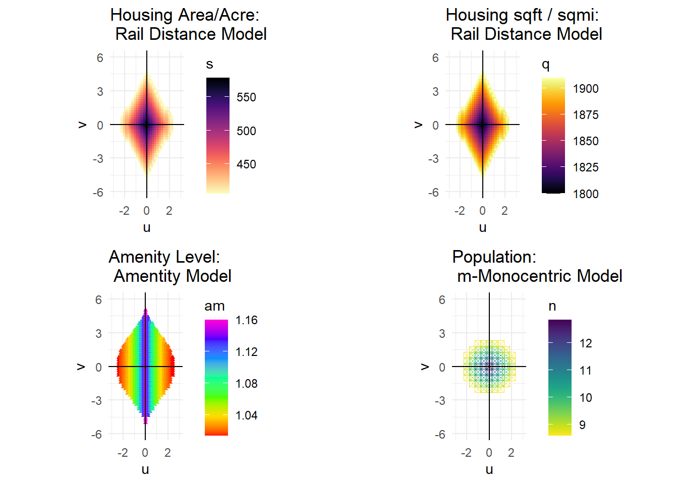
I extended the work of (Wu and Plantinga 2003) using R and certain equation modifications to investigate how the addition of a light rail line would influence a city. First, I tried to replicate their city without any parks using their parameters. Second, I made some modifications to get the city to a scale that I could represent graphically. Third, I modeled the light rail as an amenity to see the influence it has on the city. Finally, I modeled the light rail so that it reduced travel costs for the citizens close to it instead of providing an amenity value. The parameters I used where nearly identical to the (Wu and Plantinga 2003) parameters; however I did have to make some minor modifications. The given utility produced a much larger area then was graphically tractable, so I increased it to 6,000 for all the models excluding the original monocentric model which uses the original utility value. The transport cost for the rail is set to half of the normal transport costs (t¬¬rail=$500). The original parameters are shown in Table 1.
Wu, Jun Jie, and Andrew J. Plantinga. 2003. “The Influence of Public Open Space on Urban Spatial Structure.” Journal of Environmental Economics and Management 46 (2): 288–309. https://doi.org/10.1016/S0095-0696(03)00023-8.
This is an R Markdown Notebook. When you execute code within the notebook, the results appear beneath the code.
Try executing this chunk by clicking the Run button within the chunk or by placing your cursor inside it and pressing Ctrl+Shift+Enter.
library("nleqslv")
#library(circlize)
#budget
y <- 40000
#distance from center (miles) vector
x <- c(0:25)
#transportation cost 50 cents a mile by 320 days
t <- 1000
#housing price per sqft vector
p <- c(0:25)
#housing consumption (sqft) by mile vector
q <- c(0:25)
#general good
g <- c(0:25)
#utility level
V <- 2702
#alpha for Cobb Douglas
al <- .5
#beta for development cobb-douglas
bt <- 4/3
#capital
c0 <- 0
#land acres
l <- .5
#interest
i <- .03
#land rent/acre
r <- c(0:25)
#Housing floor space / acre
s <- c(0:25)
#ag rent
ag <- 1000
The equations are also nearly identical to the (Wu and Plantinga 2003) equations. I used the equations and the given parameters to calculate the optimal values at each point (u,v) for housing price (p), housing consumption (q), good consumption (g), land rent (r), housing floor space per area (s), and amenity. These optimal equations naturally satisfy the equilibrium conditions : no house moves because house prices are bid up to their maximum, no business profits because land rents are bid up to the max, the price that households are willing to pay is equal to the price businesses are willing to accept, and the floor space equals the total supply. The final equilibrium conditions that the land rent is equal to the agriculture rent at the city boundary is solved for numerically in the model.
#monocentric original model parameters

u <- c(1:50)
v <- c(1:50)

#new u,v

i <- 0
j <- 0
ii <- 1

while(i < 51){

  j <- 0
  while(j < 51){
  u[ii] <- i - 25
  v[ii] <- j - 25
  j <- j+1
  ii <- ii+1
  }

  i <- i +1

  }


#finding x for various u,v
x <- sqrt(u^2+v^2)

#finding the price for various x
p <- (al^al*(1-al)^(1-al)*(y-t*x)/V)^(1/al)

#optimal q
q <- al*(y-t*x)/p

#optimal g
g <- (1-al)*(y-t*x)


#theta some funciton of beta
ph <- ((bt-1)^((bt-1)/bt))/bt

#optimal r

r <- (ph*p)^(bt/(bt-1))

r1 <- ((ph*al)^al * (1-al)^(1-al) * (y-t*x)/V)^(bt/(al*(bt-1)))

#optimal s
s <- (p/bt)^(1/(bt-1))

s1 <- (bt-1)^(-1/bt) * (r)^(1/bt)

#Utility Value

U <- q^al*g^(1-al)


#population n s(floorspaceperacre/ floorspace per household * (size of square (sqmi)) * acres/sqmi * fraction of housing in area)
n <- s/q * 1 * 640 * .25


dfsc <- data.frame(u,v,x,p,g,q,s,r,U,n)

#delete values where ag rent exceeds land rent
dfsc1 <- dfsc[(dfsc$r > ag),]

head(dfsc1,20)
##       u  v        x         p        g        q        s        r    U
## 127 -23 -1 23.02173  9.870889 8489.136 860.0174 405.7444 1001.264 2702
## 128 -23  0 23.00000  9.896170 8500.000 858.9181 408.8700 1011.562 2702
## 129 -23  1 23.02173  9.870889 8489.136 860.0174 405.7444 1001.264 2702
## 173 -22 -6 22.80351 10.126259 8598.246 849.1039 438.0572 1108.970 2702
## 174 -22 -5 22.56103 10.413844 8719.486 837.2975 476.4496 1240.418 2702
## 175 -22 -4 22.36068 10.654498 8819.660 827.7875 510.2498 1359.114 2702
## 176 -22 -3 22.20360 10.845098 8898.198 820.4811 538.1263 1459.008 2702
## 177 -22 -2 22.09072 10.983114 8954.639 815.3097 558.9336 1534.708 2702
## 178 -22 -1 22.02272 11.066684 8988.642 812.2255 571.7897 1581.954 2702
## 179 -22  0 22.00000 11.094668 9000.000 811.2004 576.1383 1598.016 2702
## 180 -22  1 22.02272 11.066684 8988.642 812.2255 571.7897 1581.954 2702
## 181 -22  2 22.09072 10.983114 8954.639 815.3097 558.9336 1534.708 2702
## 182 -22  3 22.20360 10.845098 8898.198 820.4811 538.1263 1459.008 2702
## 183 -22  4 22.36068 10.654498 8819.660 827.7875 510.2498 1359.114 2702
## 184 -22  5 22.56103 10.413844 8719.486 837.2975 476.4496 1240.418 2702
## 185 -22  6 22.80351 10.126259 8598.246 849.1039 438.0572 1108.970 2702
## 221 -21 -9 22.84732 10.074728 8576.340 851.2727 431.4036 1086.568 2702
## 222 -21 -8 22.47221 10.520197 8763.897 833.0545 491.1967 1291.872 2702
## 223 -21 -7 22.13594 10.927718 8932.028 817.3736 550.5189 1503.979 2702
## 224 -21 -6 21.84033 11.292374 9079.835 804.0679 607.4905 1715.002 2702
##             n
## 127  75.48581
## 128  76.16466
## 129  75.48581
## 173  82.54485
## 174  91.04522
## 175  98.62431
## 176 104.93868
## 177 109.68761
## 178 112.63664
## 179 113.63669
## 180 112.63664
## 181 109.68761
## 182 104.93868
## 183  98.62431
## 184  91.04522
## 185  82.54485
## 221  81.08398
## 222  94.34134
## 223 107.76348
## 224 120.88343
nrow(dfsc1$n)
## NULL
sum(dfsc1$n)
## [1] 4222601
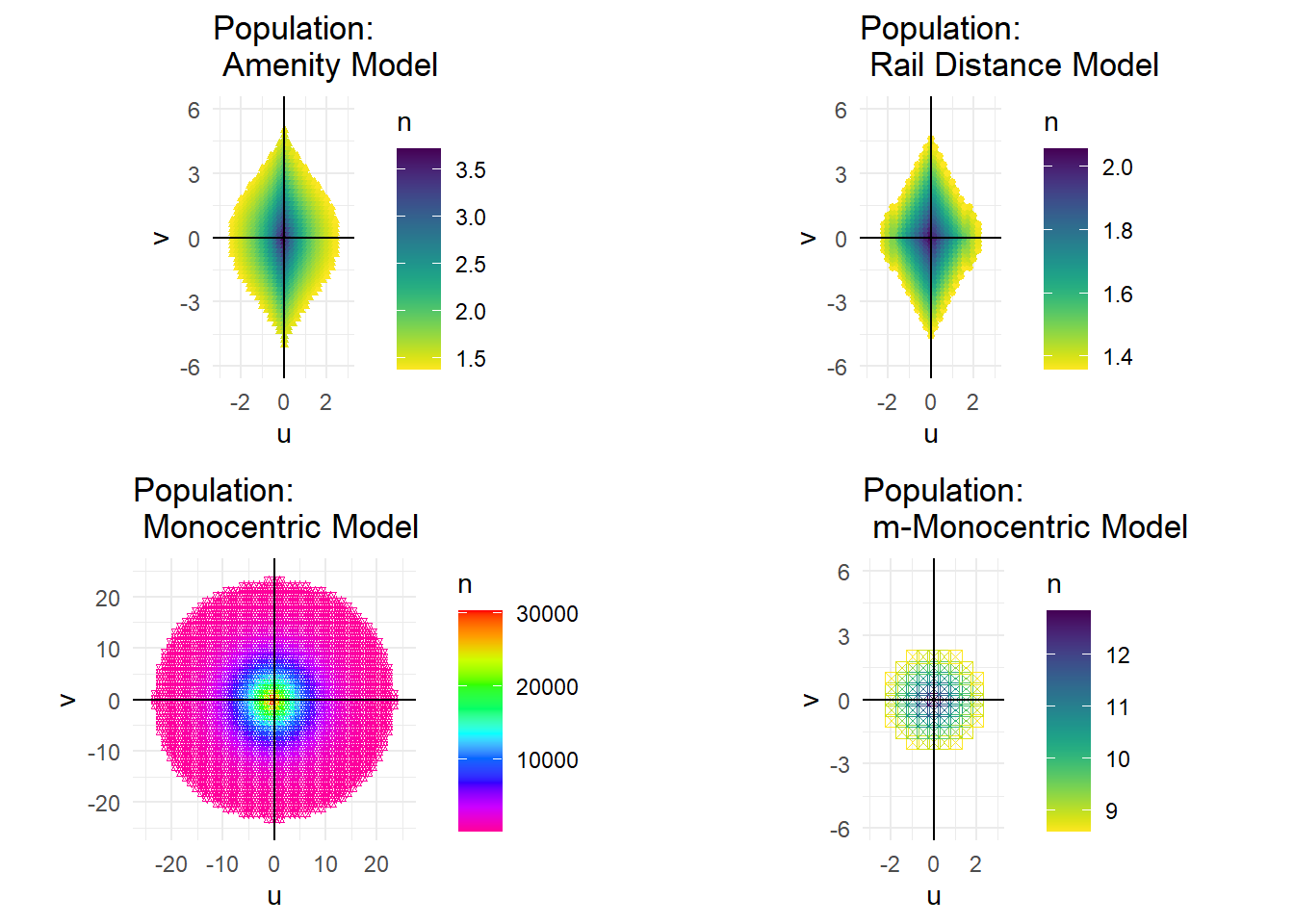
I created an x, y coordinate system with points that represented discrete area sizes. The original monocentric model has 1 square mile by 1 square mile squares, the m-Monocentric model has 0.5 square mile by 0.5 square mile squares, and both the amenity model and the rail distance model have 0.2 square mile by 0.2 square mile squares. The monocentric models’ results weren’t too interesting, so they didn’t need finely tuned points. The other models did have detailed information and empirically the 0.2 x 0.2 size squares housed at least 1 household, any smaller and their would-be fractional households. The light rail system ran right through the city center (point (0,0)) along the y axis (north- south). A horizontal line would produce similar results. Shifting the line horizontally might produce a slight variation, but probably not enough to go through the trouble of modeling. Since each point represents a specific area, I can calculate the actual values for various variables rather than their rates. Then, I can simply sum up all the points to calculate the total values for these variables on the city basis. Thus, using these discrete points, I can fully characterize each modeled city numerically. I modeled all these systems and produced the various outputs in R.
#modfied parameters

#budget
y <- 40000
#distance in the x axis
u <- c(0,0,0,0,0,1,1,1,1,1,-1,-1,-1,-1,-1,2,2,2,2,2,-2,-2,-2,-2,-2)
#distance in the y axis
v <- c(0,1,-1,2,-2,0,1,-1,2,-2,0,1,-1,2,-2,0,1,-1,2,-2,0,1,-1,2,-2)
#distance from center
x <- sqrt(u^2+v^2)

#transportation cost 50 cents a mile by 320 days
t <- 1000
#housing price per sqft vector
p <- c(0:25)
#housing consumption (sqft) by mile vector
q <- c(0:25)
#general good
g <- c(0:25)
#utility level
V <- 6000
#alpha for Cobb Douglas
al <- .5
#beta for development cobb-douglas
bt <- 4/3
#capital
c0 <- 0

#amentiy
ad <- 0.16
ng <- 1
d <- 0

#gamma for amenity
gm <- 0.5

#z distance to amentiy
z <- sqrt((u-d)^2)

#land rent/acre
r <- c(0:25)
#Housing floor space / acre
s <- c(0:25)
#ag rent
ag <- 1000
#monocentric with modified V

u <- c(1:50)
v <- c(1:50)

#new u,v

i <- 0
j <- 0
ii <- 1

while(i < 20){

  j <- 0
  while(j < 20){
  u[ii] <- i/2 - 3
  v[ii] <- j/2 - 3
  j <- j+1
  ii <- ii+1
  }

  i <- i +1

  }


#finding x for various u,v
x <- sqrt(u^2+v^2)

#finding the price for various x
p <- (al^al*(1-al)^(1-al)*(y-t*x)/V)^(1/al)

#optimal q
q <- al*(y-t*x)/p

#optimal g
g <- (1-al)*(y-t*x)


#theta some funciton of beta
ph <- ((bt-1)^((bt-1)/bt))/bt

#optimal r

r <- (ph*p)^(bt/(bt-1))

r1 <- ((ph*al)^al * (1-al)^(1-al) * (y-t*x)/V)^(bt/(al*(bt-1)))

#optimal s
s <- (p/bt)^(1/(bt-1))

s1 <- (bt-1)^(-1/bt) * (r)^(1/bt)

#Utility Value

U <- q^al*g^(1-al)


#population n s(floorspaceperacre/ floorspace per household * (size of square (sqmi)) * acres/sqmi * fraction of housing in area)
n <- s/q * (.5*.5) * 640 * .25

nn <- s/q


dfscm <- data.frame(u,v,x,p,g,q,s,r,U,n,nn)

#delete values where ag rent exceeds land rent
dfscm1 <- dfscm[(dfscm$r > ag),]

head(dfscm1,20)
##       u    v        x         p        g        q        s        r    U
## 45 -2.0 -1.0 2.236068  9.903573 18881.97 1906.581 409.7883 1014.592 6000
## 46 -2.0 -0.5 2.061553  9.995318 18969.22 1897.811 421.2827 1052.714 6000
## 47 -2.0  0.0 2.000000 10.027778 19000.00 1894.737 425.4004 1066.455 6000
## 48 -2.0  0.5 2.061553  9.995318 18969.22 1897.811 421.2827 1052.714 6000
## 49 -2.0  1.0 2.236068  9.903573 18881.97 1906.581 409.7883 1014.592 6000
## 64 -1.5 -1.5 2.121320  9.963850 18939.34 1900.805 417.3163 1039.519 6000
## 65 -1.5 -1.0 1.802776 10.132139 19098.61 1884.954 438.8207 1111.548 6000
## 66 -1.5 -0.5 1.581139 10.250062 19209.43 1874.079 454.3214 1164.206 6000
## 67 -1.5  0.0 1.500000 10.293403 19250.00 1870.130 460.1090 1184.022 6000
## 68 -1.5  0.5 1.581139 10.250062 19209.43 1874.079 454.3214 1164.206 6000
## 69 -1.5  1.0 1.802776 10.132139 19098.61 1884.954 438.8207 1111.548 6000
## 70 -1.5  1.5 2.121320  9.963850 18939.34 1900.805 417.3163 1039.519 6000
## 83 -1.0 -2.0 2.236068  9.903573 18881.97 1906.581 409.7883 1014.592 6000
## 84 -1.0 -1.5 1.802776 10.132139 19098.61 1884.954 438.8207 1111.548 6000
## 85 -1.0 -1.0 1.414214 10.339326 19292.89 1865.972 466.2947 1205.293 6000
## 86 -1.0 -0.5 1.118034 10.498662 19440.98 1851.758 488.1863 1281.326 6000
## 87 -1.0  0.0 1.000000 10.562500 19500.00 1846.154 497.1460 1312.776 6000
## 88 -1.0  0.5 1.118034 10.498662 19440.98 1851.758 488.1863 1281.326 6000
## 89 -1.0  1.0 1.414214 10.339326 19292.89 1865.972 466.2947 1205.293 6000
## 90 -1.0  1.5 1.802776 10.132139 19098.61 1884.954 438.8207 1111.548 6000
##            n        nn
## 45  8.597343 0.2149336
## 46  8.879340 0.2219835
## 47  8.980675 0.2245169
## 48  8.879340 0.2219835
## 49  8.597343 0.2149336
## 64  8.781883 0.2195471
## 65  9.312075 0.2328019
## 66  9.696951 0.2424238
## 67  9.841219 0.2460305
## 68  9.696951 0.2424238
## 69  9.312075 0.2328019
## 70  8.781883 0.2195471
## 83  8.597343 0.2149336
## 84  9.312075 0.2328019
## 85  9.995748 0.2498937
## 86 10.545358 0.2636339
## 87 10.771497 0.2692874
## 88 10.545358 0.2636339
## 89  9.995748 0.2498937
## 90  9.312075 0.2328019
nrow(dfscm1)
## [1] 69
sum(dfscm1$n)
## [1] 675.1
#Amenitiy City Model


#new u,v

i <- 0
j <- 0
ii <- 1

while(i < 61){

  j <- 0
  while(j < 61){
  u[ii] <- i/5 - 6
  v[ii] <- j/5 - 6
  j <- j+1
  ii <- ii+1
  }

  i <- i +1

  }


#finding x for various u,v
x <- sqrt(u^2+v^2)

#finding distance to rail
z <- sqrt((u-d)^2)


#amentiy distribution
am <- 1 + ad*(exp(-ng*z))

#finding the price for various u,v
p <- (al^al*(1-al)^(1-al)*am^gm*(y-t*x)/V)^(1/al)


#optimal q
q <- al*(y-t*x)/p

#optimal g
g <- (1-al)*(y-t*x)

#optimal s
s <- (p/bt)^(1/(bt-1))

#optimal r
r <- p*s - s^(bt)

#population n s(floorspaceperacre/ floorspace per household * (size of square (sqmi)) * acres/sqmi * fraction of housing in area)
n <- s/q * (.2*.2) * 640 * .25

nn <- s/q

dfuva <- data.frame(u,v,x,z,p,g,q,s,r,am,n,nn)
dfuva1 <- dfuva[(dfuva$r > ag),]
dfuva1[(dfuva1$v > 4),]
##         u   v        x   z         p        g        q        s        r
## 1821 -0.2 4.2 4.204759 0.2 10.063511 17897.62 1778.467 429.9642 1081.737
## 1822 -0.2 4.4 4.404543 0.2  9.951489 17797.73 1788.449 415.7651 1034.370
## 1882  0.0 4.2 4.200000 0.0 10.324322 17900.00 1733.770 464.2677 1198.312
## 1883  0.0 4.4 4.400000 0.0 10.209289 17800.00 1743.510 448.9214 1145.792
## 1884  0.0 4.6 4.600000 0.0 10.094900 17700.00 1753.361 434.0001 1095.297
## 1885  0.0 4.8 4.800000 0.0  9.981156 17600.00 1763.323 419.4945 1046.760
## 1886  0.0 5.0 5.000000 0.0  9.868056 17500.00 1773.399 405.3951 1000.115
## 1943  0.2 4.2 4.204759 0.2 10.063511 17897.62 1778.467 429.9642 1081.737
## 1944  0.2 4.4 4.404543 0.2  9.951489 17797.73 1788.449 415.7651 1034.370
##            am        n        nn
## 1821 1.130997 1.547271 0.2417612
## 1822 1.130997 1.487824 0.2324725
## 1882 1.160000 1.713787 0.2677793
## 1883 1.160000 1.647881 0.2574813
## 1884 1.160000 1.584158 0.2475247
## 1885 1.160000 1.522560 0.2379000
## 1886 1.160000 1.463026 0.2285978
## 1943 1.130997 1.547271 0.2417612
## 1944 1.130997 1.487824 0.2324725
nrow(dfuva1)
## [1] 727
sum(dfuva1$n)
## [1] 1379.978
#Rail Model

#values for u,v,x, and z are the same as above


#convinence penalty for taking train
cf <- 1.1

#transportation distance rail traveled and travel to rail
zz <- z+abs(v)

#cost to travel by rail
tr <- 500

#rail and commute travel cost
rtc <- (tr*abs(v)+t*abs(u))

#optimal price per square foot


p <- (al^al*(1-al)^(1-al)*(y-rtc)/V)^(1/al)


#optimal q
q <- al*(y-(rtc))/p

#optimal g
g <- (1-al)*(rtc)

#optimal s
s <- (p/bt)^(1/(bt-1))

#optimal r
r <- p*s - s^(bt)

#population n s(floorspaceperacre/ floorspace per household * (size of square (sqmi)) * acres/sqmi * fraction of housing in area)
n <- s/q * (.2*.2) * 640 * .25

nn <- s/q

#rail customers dataframe
dfr1 <- data.frame(u,v,x,z,zz,p,g,q,s,r,n,nn,rtc)

#removes all values for people more than 1.75 miles from the train
dfr1 <- dfr1[(dfr1$z <= 1.75),]
dfr1 <- dfr1[(dfr1$r > ag),]

#optimal price per square foot


p <- (al^al*(1-al)^(1-al)*(y-t*x)/V)^(1/al)


#optimal q
q <- al*(y-t*x)/p

#optimal g
g <- (1-al)*(y-t*x)

#optimal s
s <- (p/bt)^(1/(bt-1))

#optimal r
r <- p*s - s^(bt)

#population n s(floorspaceperacre/ floorspace (sqft) per household * (size of square (sqmi)) * acres/sqmi * fraction of housing in area)
n <- s/q * (.2*.2) * 640 * .25

nn <- s/q

rtc <- t*x

#non rail customers dataframe
dfr2 <- data.frame(u,v,x,z,zz,p,g,q,s,r,n,nn,rtc)


#removes all values within 1.75 of the train
dfr2 <- dfr2[(dfr2$z > 1.75),]
dfr2 <- dfr2[(dfr2$r > ag),]

dfuv <- rbind(dfr1,dfr2)


#getting rid of land rents less than land ag
dfuv1 <- dfuv[!(dfuv$r<ag),]

nrow(dfuv1)
## [1] 577
sum(dfuv1$n)
## [1] 899.1577
#dfuv1[(dfuv1$u == 0),]
#Creating All Plots

require(ggplot2)
## Loading required package: ggplot2
## Warning: package 'ggplot2' was built under R version 4.1.2
require(grid)
## Loading required package: grid
require(gridExtra)
## Loading required package: gridExtra
## Warning: package 'gridExtra' was built under R version 4.1.2
require(RColorBrewer)
## Loading required package: RColorBrewer
require(viridis)
## Loading required package: viridis
## Warning: package 'viridis' was built under R version 4.1.2
## Loading required package: viridisLite
## Warning: package 'viridisLite' was built under R version 4.1.2
#using s (housing area/acre)
p1<-ggplot(dfuv1, aes(x = u, y = v, color = s)) +
   geom_point(size = 1, shape = 19) +
  scale_color_viridis(option = 'magma', direction = -1) +
  lims(x=c(-3,3),y=c(-6,6)) +
  coord_fixed() +
  theme_minimal() +
  geom_vline(xintercept = 0) +
  geom_hline(yintercept = 0) +
  labs(title = 'Housing Area/Acre: \n Rail Distance Model')

#using q (housing sqft for area)
p2<-ggplot(dfuv1, aes(x = u, y = v, color = q)) +
   geom_point(size = 1, shape = 19) +
  scale_color_viridis(option = 'inferno') +
  #scale_color_gradientn(colors = rainbow(10)) +
  lims(x=c(-3,3),y=c(-6,6)) +
  coord_fixed() +
  theme_minimal() +
  geom_vline(xintercept = 0) +
  geom_hline(yintercept = 0) +
  labs(title = 'Housing sqft / sqmi: \n Rail Distance Model')


#using n transportation distance
p3<-ggplot(dfuv1, aes(x = u, y = v, color = n)) +
   geom_point(size = 1, shape = 19) +
  scale_color_viridis(direction = -1) +
  lims(x=c(-3,3),y=c(-6,6)) +
  coord_fixed() +
  theme_minimal()+
  geom_vline(xintercept = 0) +
  geom_hline(yintercept = 0) +
  labs(title = 'Population: \n Rail Distance Model')

#using am transportation distance
p4<-ggplot(dfuva1, aes(x = u, y = v, color = am)) +
   geom_point(size = 1, shape = 17) +

  scale_color_gradientn(colors = rainbow(7)) +
  lims(x=c(-3,3),y=c(-6,6)) +
  coord_fixed() +
  theme_minimal()+
  geom_vline(xintercept = 0) +
  geom_hline(yintercept = 0) +
  labs(title = 'Amenity Level: \n Amentity Model')

#using population for am
p5<-ggplot(dfuva1, aes(x = u, y = v, color = n)) +
   geom_point(size = 1, shape = 17) +
  scale_color_viridis(direction = -1) +
   lims(x=c(-3,3),y=c(-6,6)) +
  coord_fixed() +
  theme_minimal()+
  geom_vline(xintercept = 0) +
  geom_hline(yintercept = 0) +
  labs(title = 'Population: \n Amenity Model')

#population for original

p6<-ggplot(dfsc1, aes(x = u, y = v, color = n)) +
   geom_point(size = 1, shape = 11) +
  scale_color_gradientn(colors = rev(rainbow(10)))+
  lims(x=c(-25,25),y=c(-25,25)) +
  coord_fixed() +
  theme_minimal()+
  geom_vline(xintercept = 0) +
  geom_hline(yintercept = 0) +
  labs(title = 'Population: \n Monocentric Model')


p7<-ggplot(dfscm1, aes(x = u, y = v, color = n)) +
   geom_point(size = 2, shape = 7) +

  scale_color_viridis(direction = -1) +
  lims(x=c(-3,3),y=c(-6,6)) +
  coord_fixed() +
  theme_minimal()+
  geom_vline(xintercept = 0) +
  geom_hline(yintercept = 0) +
  labs(title = 'Population: \n m-Monocentric Model')


p8<-ggplot(dfuv1, aes(x = u, y = v, color = nn)) +
   geom_point(size = 1, shape = 19) +
  scale_color_viridis(direction = -1) +
  lims(x=c(-3,3),y=c(-6,6)) +
  coord_fixed() +
  theme_minimal()+
  geom_vline(xintercept = 0) +
  geom_hline(yintercept = 0) +
  labs(title = 'House Density: \n Rail Distance Model')

hd4<-ggplot(dfuv1, aes(x = u, y = v, color = nn)) +
   geom_point(size = 1, shape = 19) +
  scale_color_viridis(direction = -1) +
  lims(x=c(-3,3),y=c(-6,6)) +
  coord_fixed() +
  theme_minimal()+
  geom_vline(xintercept = 0) +
  geom_hline(yintercept = 0) +
  labs(title = 'House Density: \n Rail Distance Model')

hd3<-ggplot(dfuva1, aes(x = u, y = v, color = nn)) +
   geom_point(size = 1, shape = 17) +
  scale_color_viridis(direction = -1) +
  lims(x=c(-3,3),y=c(-6,6)) +
  coord_fixed() +
  theme_minimal()+
  geom_vline(xintercept = 0) +
  geom_hline(yintercept = 0) +
  labs(title = 'House Density: \n Amenity Model')

hd2<-ggplot(dfscm1, aes(x = u, y = v, color = nn)) +
   geom_point(size = 2, shape = 7) +
  scale_color_viridis(direction = -1) +
  lims(x=c(-3,3),y=c(-6,6)) +
  coord_fixed() +
  theme_minimal()+
  geom_vline(xintercept = 0) +
  geom_hline(yintercept = 0) +
  labs(title = 'House Density: \n m-Monocentric Model')


pr4<-ggplot(dfuv1, aes(x = u, y = v, color = p)) +
   geom_point(size = 1, shape = 19) +
  scale_color_viridis(option = 'magma', direction = -1) +
  lims(x=c(-3,3),y=c(-6,6)) +
  coord_fixed() +
  theme_minimal() +
  geom_vline(xintercept = 0) +
  geom_hline(yintercept = 0) +
  labs(title = 'Housing Price: \n Rail Distance Model')

pr3<-ggplot(dfuva1, aes(x = u, y = v, color = p)) +
   geom_point(size = 1, shape = 17) +
  scale_color_viridis(option = 'magma', direction = -1) +
  lims(x=c(-3,3),y=c(-6,6)) +
  coord_fixed() +
  theme_minimal() +
  geom_vline(xintercept = 0) +
  geom_hline(yintercept = 0) +
  labs(title = 'House Price: \n Amenity Model')

pr2<-ggplot(dfscm1, aes(x = u, y = v, color = p)) +
   geom_point(size = 2, shape = 7) +
  scale_color_viridis(option = 'magma', direction = -1) +
  lims(x=c(-3,3),y=c(-6,6)) +
  coord_fixed() +
  theme_minimal() +
  geom_vline(xintercept = 0) +
  geom_hline(yintercept = 0) +
  labs(title = 'House Price: \n m-Monocentric Model')


r4<-ggplot(dfuv1, aes(x = u, y = v, color = r)) +
   geom_point(size = 1, shape = 19) +
  scale_color_viridis(option = 'magma', direction = -1) +
  lims(x=c(-3,3),y=c(-6,6)) +
  coord_fixed() +
  theme_minimal() +
  geom_vline(xintercept = 0) +
  geom_hline(yintercept = 0) +
  labs(title = 'Land Rent: \n Rail Distance Model')

r3<-ggplot(dfuva1, aes(x = u, y = v, color = r)) +
   geom_point(size = 1, shape = 17) +
  scale_color_viridis(option = 'magma', direction = -1) +
  lims(x=c(-3,3),y=c(-6,6)) +
  coord_fixed() +
  theme_minimal() +
  geom_vline(xintercept = 0) +
  geom_hline(yintercept = 0) +
  labs(title = 'Land Rent: \n Amenity Model')

r2<-ggplot(dfscm1, aes(x = u, y = v, color = r)) +
   geom_point(size = 2, shape = 7) +
  scale_color_viridis(option = 'magma', direction = -1) +
  lims(x=c(-3,3),y=c(-6,6)) +
  coord_fixed() +
  theme_minimal() +
  geom_vline(xintercept = 0) +
  geom_hline(yintercept = 0) +
  labs(title = 'Land Rent: \n m-Monocentric Model')
# Displaying all graphs and Saving All Graphs


#Population Density Across Urban Areas
pop_den <- grid.arrange(p5,p3,p6,p7, ncol=2, nrow = 2)
#Housing Density Across Urban Areas
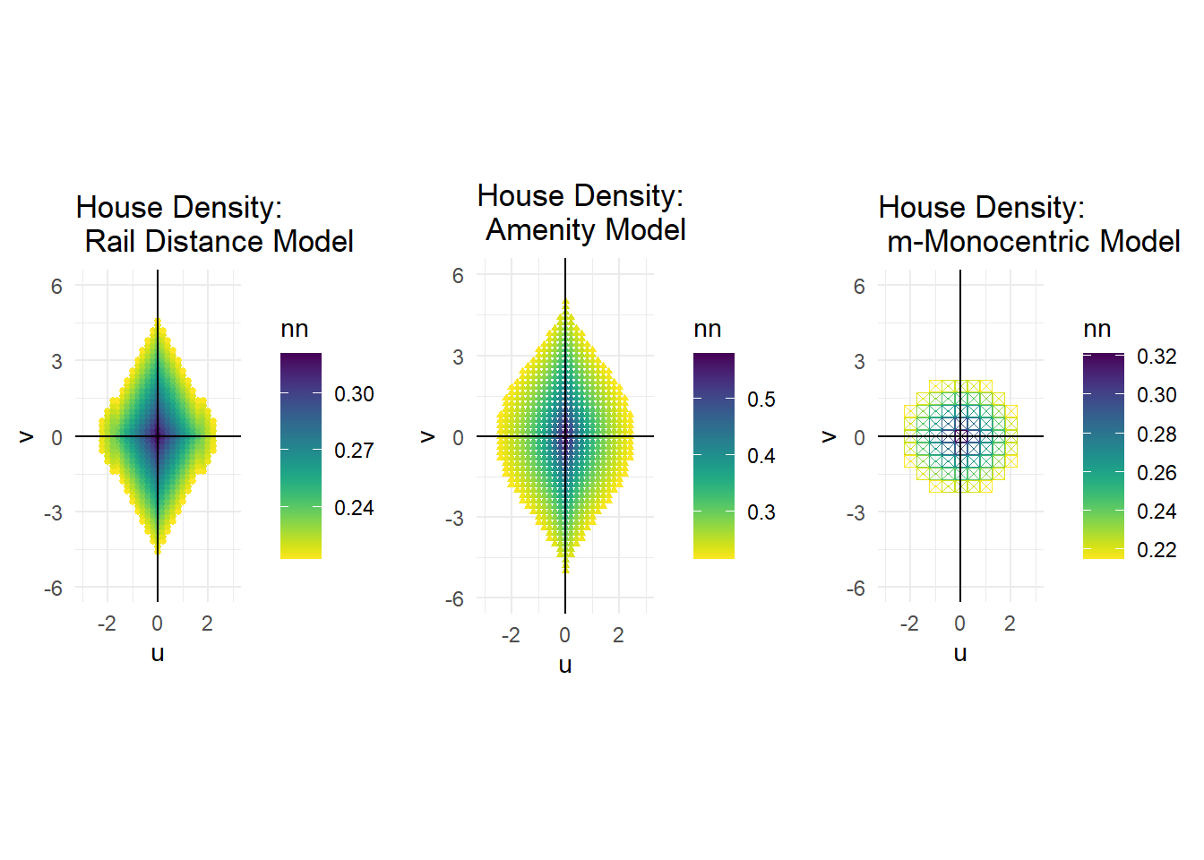
house_den <- grid.arrange(hd4,hd3,hd2,ncol =3, nrow =1)
#Housing Prices Across Urban Areas
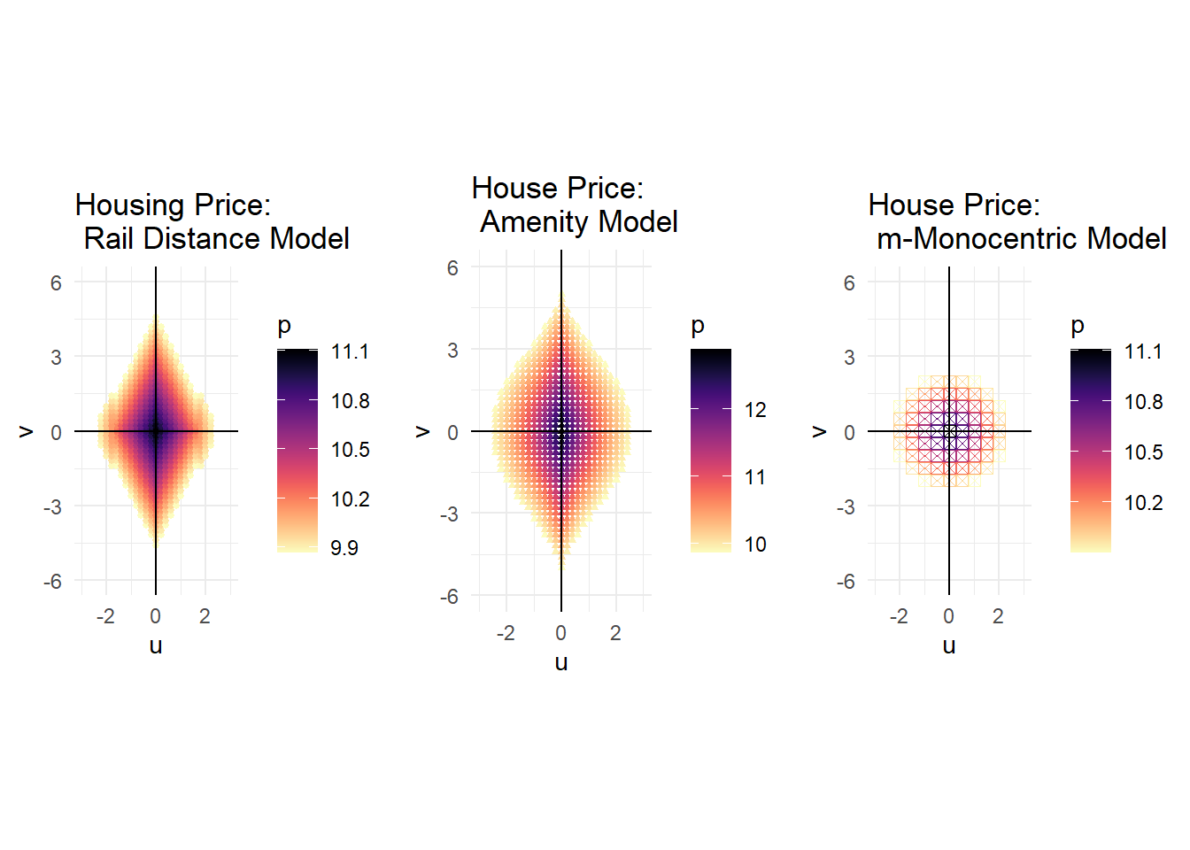
price_grid <- grid.arrange(pr4,pr3,pr2, ncol =3, nrow =1)
#Land Values across Urban Areas
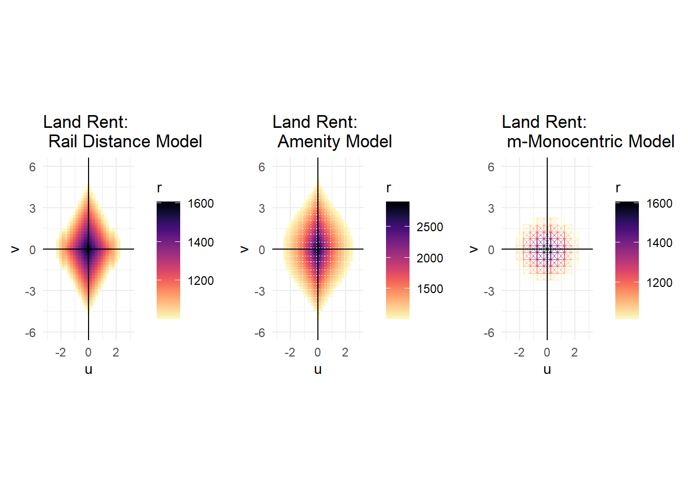
lv_grid <- grid.arrange(r4,r3,r2,ncol =3, nrow =1)
#comparisons
comp_grid <- grid.arrange(p1,p2,p4,p7, ncol=2, nrow = 2)
ggsave(filename = "pop_den.pdf", pop_den)
## Saving 7 x 5 in image
ggsave(filename = "house_den.pdf", house_den)
## Saving 7 x 5 in image
ggsave(filename = "price_grid.pdf", price_grid)
## Saving 7 x 5 in image
ggsave(filename = "lv_grid.pdf", lv_grid)
## Saving 7 x 5 in image
ggsave(filename = "comp_grid.pdf", comp_grid)
## Saving 7 x 5 in image
library(formattable)
## Warning: package 'formattable' was built under R version 4.1.2
#Number of People who take rail vs. commute
rc <- nrow(dfr1)
cc <- nrow(dfr2)
rails <- c(0,0,.10,0)
rails[4] <- round(rc/(rc+cc),4)


#Transportation Expenditures

c_trans1 <- round(sum(dfsc1$x*1000),0)
c_trans2 <- round(sum(dfscm1$x*1000),0)
c_trans3 <- round(sum(dfuva1$x)*1000,0)
c_trans4 <- round(sum(dfuv1$rtc),0)

c_trans <- rbind(c_trans1,c_trans2,c_trans3,c_trans4)


#Transportation Energy Use and GHG Emissions 120.429 MBTU/ gal, cars average 27 mpg (EIA https://www.eia.gov/energyexplained/index.php?page=about_energy_units)
#light rail every 15 mins for 12.5 hours 50 times every day. About 1 cars going 30 mph. Goes 1125 miles a day.
#64.642 MBTU/mile (http://www.rtd-fastracks.com/media/uploads/se/Energy_Tech_Report_0514_-_061814_vers.pdf)

e_trans1 <- sum(dfsc1$x*dfsc1$n*365*2*120.429/27)
e_trans2 <- sum(dfscm1$x*dfscm1$n*365*2*120.429/27)
e_trans3 <- sum(dfuva1$x*dfuva1$n*365*2*120.429/27)*.9 + 375*365*64.642
e_trans4 <- sum(dfr2$x*dfr2$n*365*2*120.429/27) + sum(dfr1$z*dfr1$n*365*2*120.429/27) + 375*365*64.642

e_trans <- rbind(e_trans1,e_trans2,e_trans3,e_trans4)

e_trans <- round(e_trans/1000,0)

# GHG of trans 8.887 kg CO2 / gallon

ghg_trans1 <- round(sum(dfsc1$x*dfsc1$n*365*2*8.887/(27*1000)),0)
ghg_trans2 <- round(sum(dfscm1$x*dfscm1$n*365*2*8.887/(27*1000)),0)
ghg_trans3 <- round((sum(dfuva1$x*dfuva1$n*365*2*8.887/(27*1000)))*.9 + 375*365*64.642/1000*((.85/3.41214/1000)/2204.6),0)
ghg_trans4 <- round(sum(dfr2$x*dfr2$n*365*2*8.887/(27*1000)) + sum(dfr1$z*dfr1$n*365*2*8.887/(27*1000)) + 375*365*64.642/1000*((.85/3.41214/1000)/2204.6),0)

tCO2_trans <- rbind(ghg_trans1,ghg_trans2,ghg_trans3,ghg_trans4)

#Residenital Energy Use and GHG Emissions 40 MBTU/sq ft (https://www.jchs.harvard.edu/blog/us-households-are-using-less-energy/)


e_res1 <- sum(dfsc1$q)*40
e_res2 <- sum(dfscm1$q)*40
e_res3 <- sum(dfuva1$q)*40
e_res4 <- sum(dfuv1$q)*40

e_res <- rbind(e_res1,e_res2,e_res3,e_res4)

e_res <- round(e_res/1000,0)

#GHG .85 lb CO2 / kwh https://data.austintexas.gov/Utilities-and-City-Services/Carbon-Intensity/hetr-8wqd
# 3.41214 MBTU/kwh 2204.6 metric tons per pound

tCO2e_res <- round(e_res*(.85/(3.41214/1000))/2204.6,0)

#Total energy and GHG
e_total <- e_res + e_trans

tCO2e_total <- tCO2e_res + tCO2_trans


#Total Land Area of the City

la1 <- nrow(dfsc1)*1
la2 <- nrow(dfscm1)*(.5*.5)
la3 <- nrow(dfuva1)*(.2*.2)
la4 <- nrow(dfuv1)*(.2*.2)

la <- rbind(la1,la2,la3,la4)


#Total Population


n1 <- round(sum(dfsc1$n),0)
n2 <- round(sum(dfscm1$n),0)
n3 <- round(sum(dfuva1$n),0)
n4 <- round(sum(dfuv1$n),0)

nt <- rbind(n1,n2,n3,n4)

#Utility
tU <- c(2700,6000,6000,6000)

s1 <- data.frame(rails, c_trans, e_trans, tCO2_trans, e_res, e_total, tCO2e_total, la, nt, tU)
rownames(s1) <- c('Moncentric', 'Monocentric Modified', 'Amenity','Rail Distance')
colnames(s1) <- c('% rail travel', '$_trans', 'MMBTU_trans', 'tCO2e_trans', 'MMBTU_res', 'MMBTU_total', 'tCO2e_total', 'City sqmi', 'Pop', 'Util' )


s2 <- s1[,2:8]/s1$Pop
colnames(s2) <- c('$_trans/house', 'MMBTU_trans/house', 'tCO2e_trans/house', 'MMBTU_res/house', 'MMBTU_total/house', 'tCO2e_total', 'Acres/house' )
s2$`Acres/house` <- s2$`Acres/house`*640*.25
s2 <- round(s2,2)
s2
##                      $_trans/house MMBTU_trans/house tCO2e_trans/house
## Moncentric                    6.07             25.71              1.90
## Monocentric Modified        159.06              4.88              0.36
## Amenity                    1133.73             12.26              0.43
## Rail Distance              1014.81             12.48              0.19
##                      MMBTU_res/house MMBTU_total/house tCO2e_total Acres/house
## Moncentric                      0.01             25.72        1.90        0.06
## Monocentric Modified            7.66             12.54        1.23        4.09
## Amenity                        37.40             49.66        4.66        3.37
## Rail Distance                  48.12             60.61        5.63        4.11
s1$`$_trans` <- prettyNum(s1$`$_trans`, big.mark = ',')
s1$MMBTU_trans <- prettyNum(s1$MMBTU_trans, big.mark =',')
s1$MMBTU_res <- prettyNum(s1$MMBTU_res, big.mark =',')
s1$MMBTU_total <- prettyNum(s1$MMBTU_total, big.mark = ',')
s1$`% rail travel` <- percent(s1$`% rail travel`, digits = 1)

s3 <- s1[,c(1,2,6,7,8,9,10)]

s3
##                      % rail travel    $_trans MMBTU_total tCO2e_total City sqmi
## Moncentric                    0.0% 25,646,389 108,602,912     8015924   1669.00
## Monocentric Modified          0.0%    107,367       8,466         827     17.25
## Amenity                      10.0%  1,564,541      68,532        6428     29.08
## Rail Distance                88.6%    912,313      54,487        5064     23.08
##                          Pop Util
## Moncentric           4222601 2700
## Monocentric Modified     675 6000
## Amenity                 1380 6000
## Rail Distance            899 6000
# Saving Files as pdfs

# pdf("city_data.pdf", height=2, width=8.5)
# grid.table(s3)
# dev.off()

# pdf("per_capita_data.pdf", height=2, width=13)
# grid.table(s2)
# dev.off()
#Solving for q and g using non-linear solver

i <- 1

while(i <= 16){


fn <- function(j) {

    a <- j[1]^al *j[2]^(1-al)-V
    b <- y-t*x[i]-p[i]*j[1]-j[2]


    return(c(a,b))

}

result <- nleqslv(c(500,10000), fn)
result$x[1] <- q[i]
result$x[2] <- g[i]

i <- i+1

}

head(data.frame(x,p,q,g),20)
##           x        p        q        g
## 1  8.485281 6.897066 2284.647 15757.36
## 2  8.345058 6.958579 2274.526 15827.47
## 3  8.207314 7.019270 2264.672 15896.34
## 4  8.072174 7.079070 2255.086 15963.91
## 5  7.939773 7.137904 2245.773 16030.11
## 6  7.810250 7.195695 2236.737 16094.88
## 7  7.683749 7.252362 2227.981 16158.13
## 8  7.560423 7.307820 2219.511 16219.79
## 9  7.440430 7.361983 2211.331 16279.78
## 10 7.323933 7.414759 2203.448 16338.03
## 11 7.211103 7.466054 2195.865 16394.45
## 12 7.102112 7.515771 2188.590 16448.94
## 13 6.997142 7.563810 2181.629 16501.43
## 14 6.896376 7.610069 2174.988 16551.81
## 15 6.800000 7.654444 2168.675 16600.00
## 16 6.708204 7.696831 2162.695 16645.90
## 17 6.621178 7.737123 2157.056 16689.41
## 18 6.539113 7.775215 2151.766 16730.44
## 19 6.462198 7.811001 2146.831 16768.90
## 20 6.390618 7.844379 2142.259 16804.69
- Posted on:
- March 3, 2019
- Length:
- 19 minute read, 4027 words
- Categories:
- Systems Modeling
- Tags:
- Systems Modeling Simulation cities