Quadratic Programming Examples and Algorithms

library(gurobi)

library(tictoc)
library(Matrix)
library(ggplot2)

#library(matlib)
library(MASS)

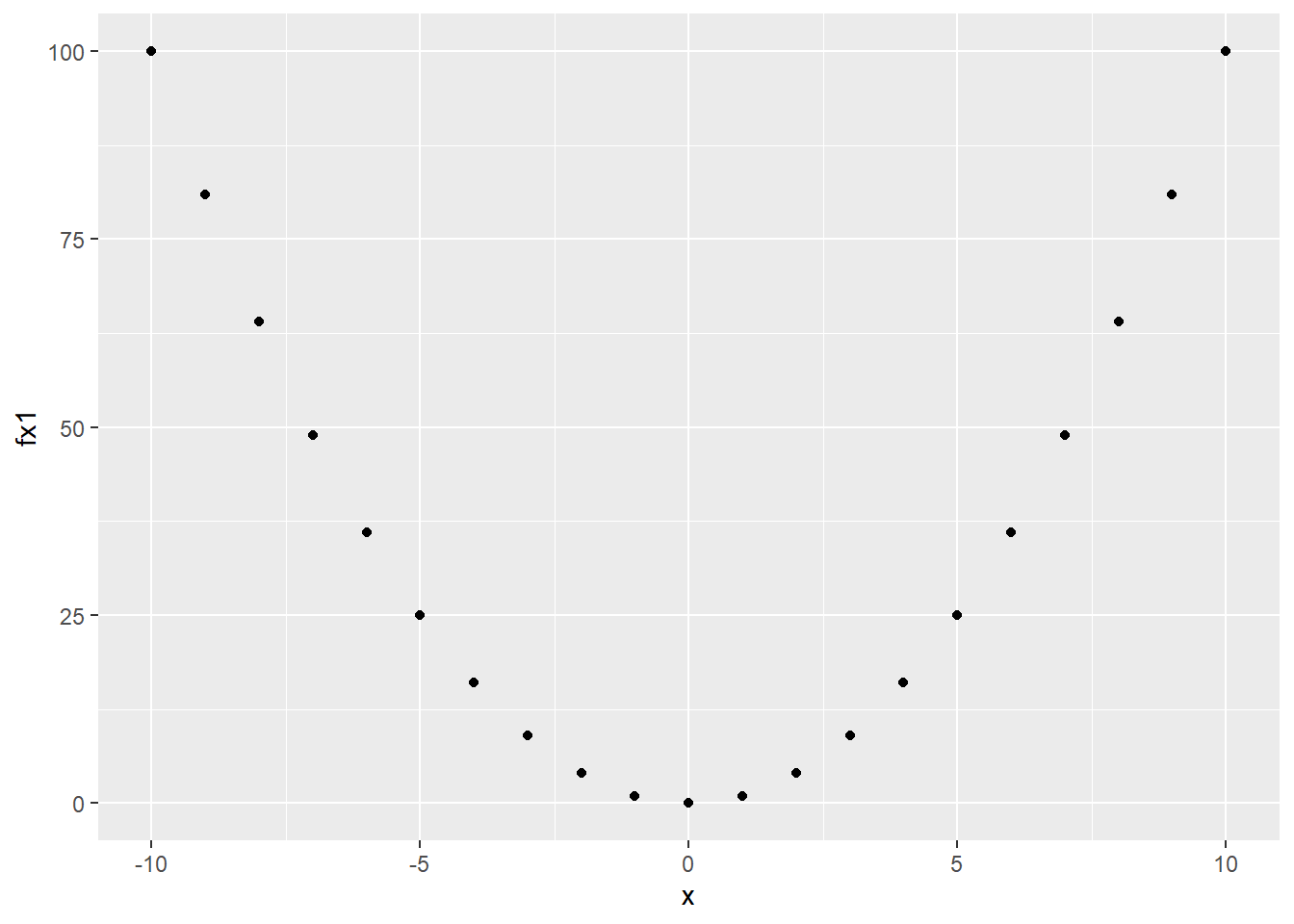
x <- c(-10:10)
fx1 <- x^2
xi <- 10
lambda <- 0.2
xit <- xi

fx <- xit^2
dfx <- 2*xit

gd <- data.frame('x' = xit, 'fx' = fx, 'dfx' = dfx)



while(dfx < -10^-50 | dfx > 10^-50){
xit <- xit - lambda*dfx
fx <- xit^2
dfx <- 2*xit
gd <- rbind(gd, c(xit,fx,dfx))

}

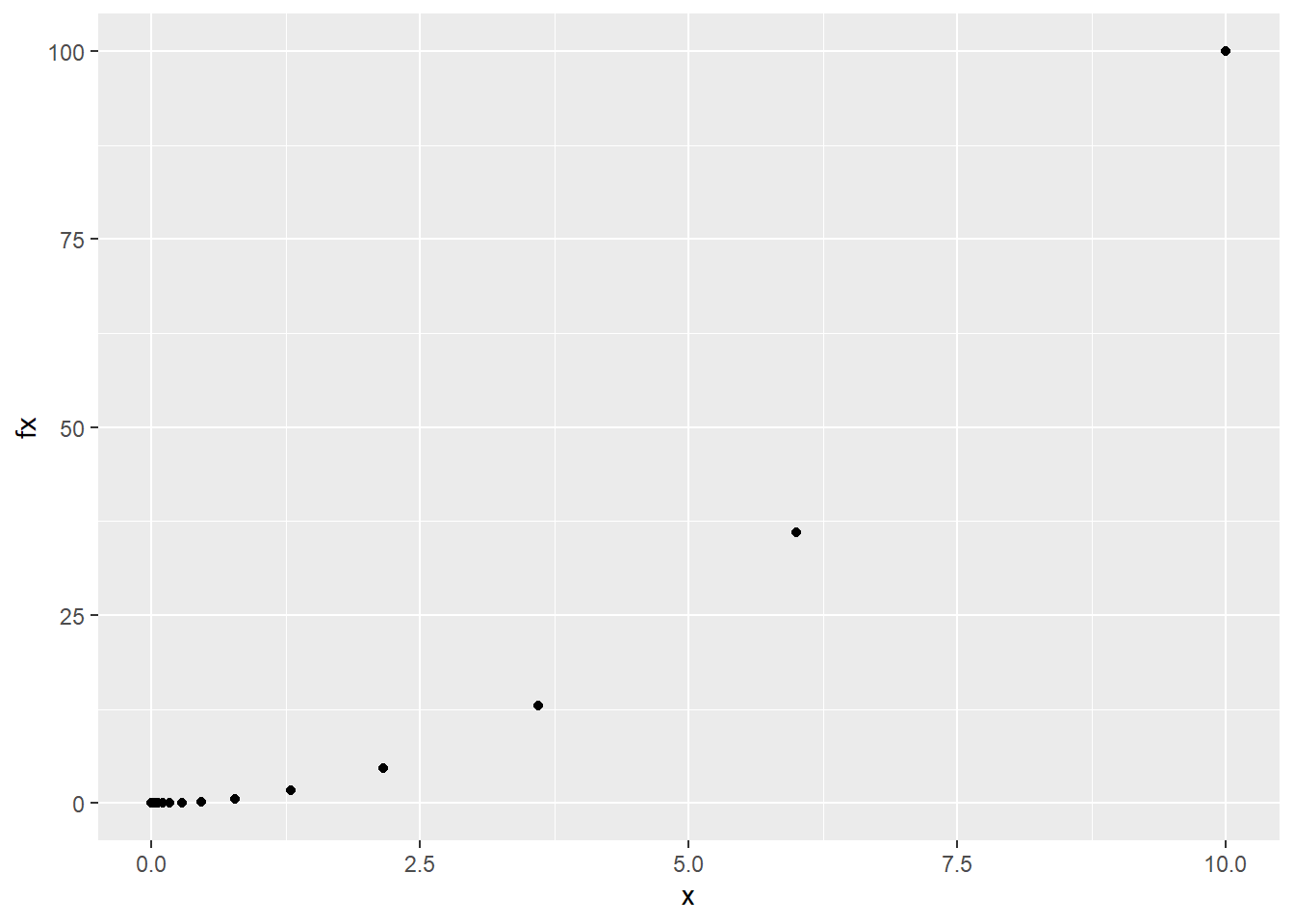
head(gd)

tail(gd)

qplot(x = x, y = fx1)

qplot(x,fx, data = gd)

constr1 <- c(1,1,1,0)
constr2 <- c(1,0,0,1)


A <- rbind(constr1,constr2)

m <- nrow(A)
n <- ncol(A)


b <- matrix(c(5,3),nrow =m)
c <- matrix(c(-8,-16,0,0), nrow = n)
Q <- rbind(c(2,0,0,0),c(0,8,0,0),c(0,0,0,0),c(0,0,0,0))
#inital x values (xi) given by slacks = RHS
xi <- matrix(c(1,1,0.5,0.5), nrow =n)

m <- nrow(A)
n <- ncol(A)

I <- diag(n)
z1 <- matrix(rep(0,n*n), nrow = n)
z2 <- matrix(rep(0,m*m), nrow = m)
z3 <- matrix(rep(0,m*n), nrow = m)
y <- matrix(rep(1,m), nrow = n)
#The complimentary slackness modifier 1/t eventually goes to 0 as t >>>> inf
t <- 9
#Step size pretty much make it up
alpha <- 0.1
#mu*x = 0 in complemntariy slackness condition , mu >0 is dual condition mu correspond to dual variables, 
#using fancy vectors this gives Xd*mu = XM1 = 1/t where t >>>> inf 
x <- xi
mu <- x/t
mu_minus_c <- mu - c - Q%*%x
#Gives lagrangian multipliers for constraints
#Solving c+A*lamda-mu = 0 gives initial lambda
lambda <- ginv(t(A))%*%(mu_minus_c)


#combined vector having values of x, lambda, and mu useful when adding the search direction
w <- rbind(x, lambda, mu)


#This is the KKT condition stationarity, at optimality this derivative should  be 0,
#Using the lagrangian cx+lambda*Ax-mu >> c+A*lambda-mu
c_plus_tA <- Q%*%x+c+t(A)%*%lambda-mu

#This is the KKT condition primal feasiblity, this should always be 0 Ax-b=0 
A_times_x_minus_b <- A%*%x-b

#This is the modfied complimentary condtion XM1 -1/t = 0 X is the diag(x) and M is diag(mu) 1/t >>> 0 as t gets larger
x_times_mu_minus_y_over_t <- x*mu-y/t

#The right hand side of the search direction iteration given from the Newton-Raphson Method
#Combines the vectors above
B <- rbind(c_plus_tA,A_times_x_minus_b,x_times_mu_minus_y_over_t)

objective <- 0.5*t(x)%*%Q%*%x+t(c)%*%x
error <- norm(B,'2')

iteration_list <- data.frame('x1' = x[1], 'x2' = x[2], 'x3' = x[3], 'x4' = x[4], 'objective' = objective, 'error' = error)

#loop



while(error > 10^-12){
t <- t*9

Xd = Diagonal(n = n, x)

Mud = Diagonal(n = n, mu) 


#The left hand side matrix of the search direction iteration, it containtes information from the A, x, and mu vectors and matricies of 1s or 0s to make the math make sense

C <- rbind(cbind(Q,t(A),-I),cbind(A,z2,z3), cbind(Mud,t(z3), Xd))

#The right hand side of the search direction iteration given from the Newton-Raphson Method
#This contains the objective function costs, the RHS values, as well as the A, x, and mu vectors. 
#It also has the complimentary condition represented by t
B <- rbind(Q%*%x+c+t(A)%*%lambda-mu,A%*%x-b,x*mu-y/t)


#solving the systems of equations with C and B gives the search direction as you move closer and closer to solving the complimentary condition in the KKT conditions
dw = solve(-C,B)


#update your w vector which is just a list of the x, mu, and lambda vectors using the search direction
w <- w + alpha*dw

x <- w[1:n]

lambda <- w[(n+1):(n+m)]

mu <- w[(n+m+1):length(w)]

#calculate the objective function from the x values and the error. Remember if this satisifies all the KKT conditions then the B vector will be 0.
objective <- 0.5*t(x)%*%Q%*%x+t(c)%*%x
error <- norm(B,'2')
iteration_list <- rbind(iteration_list,c(x,objective,error))

}

head(iteration_list)

tail(iteration_list)

#Another example from http://fourier.eng.hmc.edu/e176/lectures/ch3/node19.html, but don't have answers 



#Work out matricies in Wolfram Alpha

#Idea given A,b,c and intial value of x; find optimal x that minimizes c'*x

constr1 <- c(2,1,1,0,0)
constr2 <- c(6,5,0,1,0)
constr3 <- c(2,5,0,0,1)

A <- rbind(constr1,constr2, constr3)

b <- matrix(c(18,60,40),nrow =3)
c <- matrix(c(-8,-16,0,0,0), nrow = 5)
Q <- rbind(c(2,1,0,0,0),c(1,2,0,0,0),c(0,0,0,0,0),c(0,0,0,0,0),c(0,0,0,0,0))

rm(A,b,c,Q,constr1,constr2,constr3)