Basics of Markov Chains
By Erick Jones in ORIE Basics
January 4, 2020
Background
This post explores how to markov chains work and how to visulaize them in R. I use a R package specifically designed to visualize markov chains. I also represent these markov chains using tables. This is a reproducible example if you have R Studio just make sure you have installed the correct packages.
library(markovchain)
## Warning: package 'markovchain' was built under R version 4.1.2
library(diagram)
#Allows the use of exponential operators in matrix
library(expm)
## Warning: package 'expm' was built under R version 4.1.2
#library(matlib)
Example
A good article about Markov Chain Monte Carlo Methods: https://towardsdatascience.com/a-zero-math-introduction-to-markov-chain-monte-carlo-methods-dcba889e0c50
Example from https://www.analyticsvidhya.com/blog/2014/07/markov-chain-simplified/
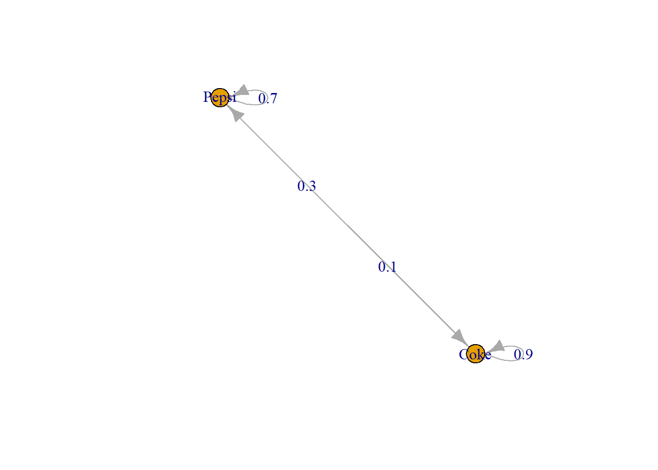
# Creating a transition matrix
trans_mat <- matrix(c(0.7,0.3,0.1,0.9),nrow = 2, byrow = TRUE)
trans_mat
##      [,1] [,2]
## [1,]  0.7  0.3
## [2,]  0.1  0.9
# create the Discrete Time Markov Chain
disc_trans <- new("markovchain",transitionMatrix=trans_mat, states=c("Pepsi","Coke"), name="MC 1")
mcDF <- as(disc_trans,"data.frame")
mcDF
##      t0    t1 prob
## 1 Pepsi Pepsi  0.7
## 2 Pepsi  Coke  0.3
## 3  Coke Pepsi  0.1
## 4  Coke  Coke  0.9
disc_trans
## MC 1
##  A  2 - dimensional discrete Markov Chain defined by the following states:
##  Pepsi, Coke
##  The transition matrix  (by rows)  is defined as follows:
##       Pepsi Coke
## Pepsi   0.7  0.3
## Coke    0.1  0.9
plot(disc_trans)
#Market Share after one month
Current_state <- c(0.55,0.45)
steps <- 1
finalState <- Current_state*disc_trans^steps #using power operator
finalState
##      Pepsi Coke
## [1,]  0.43 0.57
#Market Share after two month
Current_state <- c(0.55,0.45)
steps <- 2
finalState <- Current_state*disc_trans^steps #using power operator
finalState
##      Pepsi  Coke
## [1,] 0.358 0.642
#Markov Chain Statistical Operations
steadyStates(disc_trans)
##      Pepsi Coke
## [1,]  0.25 0.75
meanFirstPassageTime(disc_trans)
##       Pepsi     Coke
## Pepsi     0 3.333333
## Coke     10 0.000000
meanRecurrenceTime(disc_trans)
##    Pepsi     Coke
## 4.000000 1.333333
hittingProbabilities(disc_trans)
##       Pepsi Coke
## Pepsi     1    1
## Coke      1    1
meanAbsorptionTime(disc_trans)
## named numeric(0)
#absorptionProbabilities(disc_trans)
period(disc_trans)
## [1] 1
summary(disc_trans)
## MC 1  Markov chain that is composed by:
## Closed classes:
## Pepsi Coke
## Recurrent classes:
## {Pepsi,Coke}
## Transient classes:
## NONE
## The Markov chain is irreducible
## The absorbing states are: NONE
Manually Calculating Markov Chains
https://www.probabilitycourse.com/chapter11/11_2_1_introduction.php
Chapman-Kolmogorov Equation:
P^(n) = P^n p_ij^(m+n) = P(X_m+n = j | X_0 = i) = sum(p_ik^(m)*p_kj^(n))
#Probabilty Space after 5 steps
steps <- 5

Current_state%*%(trans_mat%^%steps)
##          [,1]     [,2]
## [1,] 0.273328 0.726672
#Mean Return and Mean Hitting Times using Recursive Equations
#r_l = 1 + sum(t_k*p_lk)
#t_l = 0; t_k = 1 + sum(t_j*p_kj)

#Given X_0 = Coke time until pepsi first time, t_pepsi = 0
# t_coke = 1 + 1/10*t_pepsi + 9/10t_coke
t_coke <- solve(1/10,1)
#r_pepsi = 1 + 7/10*t_pepsi + 3/10*t_coke
r_pepsi <- 1 + 3/10*t_coke

meanFirstPassageTime(disc_trans)
##       Pepsi     Coke
## Pepsi     0 3.333333
## Coke     10 0.000000
t_coke
## [1] 10
meanRecurrenceTime(disc_trans)
##    Pepsi     Coke
## 4.000000 1.333333
r_pepsi
## [1] 4
#Steady State
#Stationary Distribtution pi = pi*P, sum(pi) = 1 and if irreducible and aperiodic pi_j = lim(n>inf)P(X_n =j | X_0 = i)
#pi_p = 7/10pi_p+1/10pi_c; pi_c = 3/10pi_p + 9/10pi_c, pi_c+pi_p =1
A <- matrix(c(-3/10,1/10,3/10,-1/10,1,1), nrow =3, byrow = TRUE )
B <- c(0,0,1)
steadyStates(disc_trans)
##      Pepsi Coke
## [1,]  0.25 0.75
# Solve(A,B)


#rm(Current_state, disc_trans, finalState,steps,trans_mat)
Continous Time Markov Chains
energyStates <- c("sigma", "sigma_star")
#Must produce generator matrix from a transistion probablity matrix
Q <- expm::logm(disc_trans@transitionMatrix,method='Eigen')

gen <- matrix(data = c(-3, 3, 1, -1), nrow = 2, byrow = TRUE, dimnames = list(energyStates, energyStates))

molecularCTMC <- new("ctmc", states = energyStates, byrow = TRUE, generator = gen, name = "Molecular Transition Model")

statesDist <- c(0.8, 0.2)
rctmc(n = 3, ctmc = molecularCTMC, initDist = statesDist, out.type = "df", include.T0 = FALSE, T = 4)
##       states              time
## 1 sigma_star 0.450251907717093
## 2      sigma  2.81869318570598
## 3 sigma_star  2.87532378315582
steadyStates(molecularCTMC)
##      sigma sigma_star
## [1,]  0.25       0.75
Q-Learning with Liars Dice
http://gradientdescending.com/q-learning-example-with-liars-dice-in-r/
# play a round of liars dice
liars.dice.round <- function(players, control, player.dice.count, agents, game.states, reward, Q.mat, a = 1, verbose = 1){

  # set array for recording results
  y.ctrl = c(); y.state = c(); y.action = c()

  # roll the dice for each player
  if(verbose > 0) cat("\n\n")
  rolls <- lapply(1:players, function(x) sort(sample(1:6, player.dice.count[[x]], replace = TRUE)))
  if(verbose > 1) lapply(rolls, function(x) cat("dice: ", x, "\n"))
  total.dice <- sum(unlist(player.dice.count))

  # set penalty
  penalty <- sapply(1:players, function(x) 0, simplify = FALSE)

  # print dice blocks
  if(verbose > 0) Dice(rolls[[1]])

  # set up roll table
  roll.table <- roll.table.fn(rolls)

  # initial bid
  if(verbose > 0) cat("place first bid\nPlayer", control, "has control\n")
  if(control == a){

    dice.value <- set.dice.value("dice value: ", 6)
    dice.quantity <- set.dice.value("quantity; ", sum(roll.table))

  }else{

    # agent plays
    p1.state <- which(game.states$total == total.dice & game.states$p1 == player.dice.count[[1]] & game.states$prob_cat == total.dice)
    pars <- list(dice = rolls[[control]], total.dice = total.dice, dice.value = NULL, dice.quantity = 0, p1.state = p1.state)
    agent.action <- agents[[control]](pars = pars, Q.mat = Q.mat)
    dice.value <- agent.action$dice.value
    dice.quantity <- agent.action$dice.quantity

  }


  # calculate probability cat and determine the game state
  # action set to raise because you can't call without an initial bid
  # this could be a 3rd action (initial bid) but it's not really necessary
  player.dice.qty <- table(rolls[[1]])[as.character(dice.value)]
  player.dice.qty <- ifelse(is.na(player.dice.qty), 0, player.dice.qty) %>% unname
  prob.cat <- calc.prob(c(total.dice, player.dice.count[[1]], dice.quantity, player.dice.qty))
  p1.state <- which(game.states$total == total.dice & game.states$p1 == player.dice.count[[1]] & game.states$prob_cat == prob.cat)
  p1.action <- "raise"

  # storing states for Q iteration
  y.ctrl = c(); y.state = c(); y.action = c()

  # moving control to the next player
  # storing the previous player since if the next player calls the previous player could lose a die
  prev <- control
  control <- control %% players + 1
  if(verbose > 0) cat("dice value ", dice.value, "; dice quantity ", dice.quantity, "\n")


  # loop through each player and continue until there is a winner and loser
  called <- FALSE
  while(!called){

    # check if the player with control is still in the game - if not skip
    if(player.dice.count[[control]] > 0){
      if(control == a){

        action <- readline("raise or call (r/c)? ")

      }else{

        # the agent makes a decision
        pars <- list(dice = rolls[[control]], total.dice = total.dice, dice.value = dice.value, dice.quantity = dice.quantity, p1.state = p1.state)
        agent.action <- agents[[control]](pars = pars, Q.mat = Q.mat)
        action <- agent.action$action

      }


      # storing states for reward iteration
      if(control == 1 & !is.null(agent.action$action)){
        player.dice.qty <- table(rolls[[1]])[as.character(dice.value)]
        player.dice.qty <- ifelse(is.na(player.dice.qty), 0, player.dice.qty) %>% unname

        p1.action <- agent.action$action
        prob.cat <- calc.prob(c(total.dice, player.dice.count[[1]], dice.quantity, player.dice.qty))
        p1.state <- which(game.states$total == total.dice & game.states$p1 == player.dice.count[[1]] & game.states$prob_cat == prob.cat)
      }


      # called
      if(action %in% c("call", "c")){

        if(verbose > 0) {
          cat("player", control, "called\nRoll table\n")
          print(roll.table)
        }

        # dice are reavealed

        # check if the quantity of dice value is less or more than the total in the pool
        # if more control loses otherwise control-1 win
        if(dice.quantity > roll.table[dice.value]){

          penalty[[prev]] <- penalty[[prev]] - 1
          if(verbose > 0) cat("player", prev, "lost a die\n")

        }else{

          penalty[[control]] <- penalty[[control]] - 1
          if(verbose > 0) cat("player", control, "lost a die\n")

        }

        # for Q iteration
        y.ctrl <- c(y.ctrl, control); y.state <- c(y.state, p1.state); y.action <- c(y.action, p1.action)

        # if called use the penalty array to change states
        prob.cat <- calc.prob(c(total.dice, player.dice.count[[1]], dice.quantity, player.dice.qty))
        p1.state <- which(game.states$total == total.dice-1 & game.states$p1 == player.dice.count[[1]]+penalty[[1]] & game.states$prob_cat == prob.cat)

        # break the loop
        called <- TRUE

      }else{

        if(verbose > 0) cat("player", control, "raised\n")

        if(control == a){

          # player sets next dice value
          dice.value <- set.dice.value("dice value: ", 6)
          dice.quantity <- set.dice.value("quantity; ", sum(roll.table))

        }else{

          dice.value <- agent.action$dice.value
          dice.quantity <- agent.action$dice.quantity
        }

        # p1 state after the raise
        prob.cat <- calc.prob(c(total.dice, player.dice.count[[1]], dice.quantity, player.dice.qty))
        p1.state <- which(game.states$total == total.dice & game.states$p1 == player.dice.count[[1]] & game.states$prob_cat == prob.cat)
        if(verbose > 0) cat("dice value", dice.value, "; dice quantity", dice.quantity, "\n")
      }

      # store info for Q update
      y.ctrl <- c(y.ctrl, control); y.state <- c(y.state, p1.state); y.action <- c(y.action, p1.action)

      # set the control player to now be the previous player
      prev <- control
    }

    # next player has control
    control <- control %% players + 1
  }

  # play results and return
  play <- data.frame(y.ctrl, y.state, y.action)
  return(list(penalty = penalty, play = play))
}


# play a full game of liars dice
play.liars.dice <- function(players = 4, num.dice = 6, auto = FALSE, verbose = 1, agents, Q.mat = NULL, train = FALSE, print.trans = FALSE){

  # begin!
  if(verbose > 0) liars.dice.title()

  # setting the number of dice each player has
  ndice <- sapply(rep(num.dice, players), function(x) x, simplify = FALSE)
  players.left <- sum(unlist(ndice) > 0)

  # setting game states matrix
  game.states <- generate.game.states(players, num.dice)

  # set up reward matrix
  reward <- generate.reward.matrix(game.states)
  reward <- list(raise = reward, call = reward)

  # set Q matrix if null
  if(is.null(Q.mat)) Q.mat <- matrix(0, nrow = nrow(reward$raise), ncol = length(reward), dimnames = list(c(), names(reward)))

  # while there is at least 2 left in the game
  # who has control
  ctrl <- sample(1:players, 1)
  play.df <- data.frame()
  while(players.left > 1){

    # play a round
    results <- liars.dice.round(
      players = players,
      control = ctrl,
      player.dice.count = ndice,
      game.states = game.states,
      reward = reward,
      Q.mat = Q.mat,
      agents = agents,
      a = as.numeric(!auto),
      verbose = verbose
    )

    # update how many dice the players are left with given the
    # outcomes of the round
    for(k in seq_along(ndice)){
      ndice[[k]] <- ndice[[k]] + results$penalty[[k]]
      if(ndice[[k]] == 0 & results$penalty[[k]] == -1){
        if(verbose > 0) cat("player", k, "is out of the game\n")
      }

      # update who has control so they can start the bidding
      if(results$penalty[[k]] == -1){
        ctrl <- k
        while(ndice[[ctrl]] == 0){
          ctrl <- ctrl %% players + 1
        }
      }
    }

    # checking how many are left and if anyone won the game
    players.left <- sum(unlist(ndice) > 0)
    if(players.left == 1){
      if(verbose > 0) cat("player", which(unlist(ndice) > 0), "won the game\n")
    }

    # appending play
    play.df <- rbind(play.df, results$play)
  }

  if(print.trans) print(play.df)

  # update Q
  # rather than training after each action, training at the
  # end of each game in bulk
  # just easier this way
  if(train) Q.mat <- update.Q(play.df, Q.mat, reward)

  # return the winner and Q matrix
  return(list(winner = which(unlist(ndice) > 0), Q.mat = Q.mat))
}
Other Stochastic Processes
Martingales http://gradientdescending.com/martingale-strategies-dont-work-but-we-knew-that-simulation-analysis-in-r/ https://github.com/doehm/martingale
Bayesian Networks http://gradientdescending.com/simulating-data-with-bayesian-networks/
Other Q Learning https://www.r-bloggers.com/a-simple-intro-to-q-learning-in-r-floor-plan-navigation/ https://dataaspirant.com/2018/02/05/reinforcement-learning-r/