Decomposition Algorithms Broken Down and Explained

Teaching · IE 5301 Advanced Operations Research

Python, run with the free Gurobi licence where it uses Gurobi. Download the notebook to run it yourself. First published January 10, 2020 (in R).

Decomposition methods rest on one fact about polyhedra: every point of one is a convex combination of its extreme points (corners) plus a non-negative combination of its extreme rays (edges that run off to infinity). Benders decomposition uses that fact to add rows to a master problem, one cut per extreme point or ray. Dantzig-Wolfe decomposition uses it to add columns, one variable per extreme point. This lesson looks at the extreme points directly, then generates columns for the cutting stock problem.

To run it yourself: pip install gurobipy numpy pandas matplotlib. The free licence that comes with pip install gurobipy is enough for everything here.

import itertools
import numpy as np
import pandas as pd
import matplotlib.pyplot as plt
import gurobipy as gp
from gurobipy import GRB

Extreme points and extreme rays

Take the mixed-integer program from the Benders lesson:

\begin{aligned} \max\ 2x_1 + x_2 + 13x_3 + 7y_1 + 5y_2 \quad \text{s.t.}\quad 9x_1 + 4x_2 + 14x_3 + 35y_1 + 24y_2 &\le 80 \\ -x_1 - 2x_2 + 3x_3 - 3y_1 + 4y_2 &\le 10 \\ x \ge 0 \text{ and integer},\quad y &\ge 0 \end{aligned}

With $x$ fixed, the dual of the problem in $y$ has the region $U = \{u \ge 0 : 35u_1 - 3u_2 \ge 7,\ 24u_1 + 4u_2 \ge 5\}$ . Write it as $Gu \ge h$ , four rows.

G = np.array([[35.0, -3.0],
              [24.0,  4.0],
              [ 1.0,  0.0],
              [ 0.0,  1.0]])
h = np.array([7.0, 5.0, 0.0, 0.0])
print("G is", G.shape, "| h =", h)

G is (4, 2) | h = [7. 5. 0. 0.]

A corner is where two of the four boundary lines cross and every other constraint still holds. Try every pair. Predict: how many of the six pairs give a corner?

corners = []
for i, j in itertools.combinations(range(4), 2):
    M = G[[i, j]]
    if abs(np.linalg.det(M)) < 1e-12:
        continue
    p = np.linalg.solve(M, h[[i, j]])
    ok = np.all(G @ p >= h - 1e-9)
    print(f"rows {i},{j}: u = ({p[0]:.4f}, {p[1]:.4f})  {'corner' if ok else 'outside U'}")
    if ok:
        corners.append(p)
corners = np.array(corners)

rows 0,1: u = (0.2028, 0.0330)  corner
rows 0,2: u = (0.0000, -2.3333)  outside U
rows 0,3: u = (0.2000, 0.0000)  outside U
rows 1,2: u = (0.0000, 1.2500)  outside U
rows 1,3: u = (0.2083, 0.0000)  corner
rows 2,3: u = (0.0000, 0.0000)  outside U

A ray is a direction $d$ you can travel forever without leaving $U$ : $Gd \ge 0$ , the same rows with the right-hand side set to zero. Scale it so $d_1 + d_2 = 1$ . An extreme ray makes one of those homogeneous rows tight.

rays = []
for i in range(4):
    d = np.linalg.solve(np.array([G[i], [1.0, 1.0]]), np.array([0.0, 1.0]))
    ok = np.all(G @ d >= -1e-9)
    print(f"row {i} tight: d = ({d[0]:.4f}, {d[1]:.4f})  {'extreme ray' if ok else 'leaves U'}")
    if ok:
        rays.append(d)
rays = np.array(rays)

row 0 tight: d = (0.0789, 0.9211)  extreme ray
row 1 tight: d = (-0.2000, 1.2000)  leaves U
row 2 tight: d = (0.0000, 1.0000)  leaves U
row 3 tight: d = (1.0000, 0.0000)  extreme ray

The region, its corners and its rays.

top = (35 * 0.3 - 7) / 3                     # the steep edge where it meets u1 = 0.3
region = np.array([corners[0], corners[1], [0.3, 0.0], [0.3, top]])
fig, ax = plt.subplots(figsize=(6, 4.2))
ax.fill(region[:, 0], region[:, 1], alpha=0.2, label="dual region U")
ax.plot(corners[:, 0], corners[:, 1], "ko", label="extreme points")
for p, d, length, style in [(corners[0], rays[0], 0.4, "--"), (corners[1], rays[1], 0.07, "-")]:
    ax.annotate("", xy=p + length * d, xytext=p, arrowprops=dict(arrowstyle="->", linestyle=style, lw=1.5))
    ax.annotate(f"ray ({d[0]:.3f}, {d[1]:.3f})", p + length * d, textcoords="offset points",
                xytext=(-4, 6), ha="right", fontsize=8)
for p, offset in zip(corners, [(-6, 4), (6, -12)]):
    ax.annotate(f"({p[0]:.4f}, {p[1]:.4f})", p, textcoords="offset points", xytext=offset,
                ha="right" if offset[0] < 0 else "left", fontsize=8)
ax.set(xlim=(0.17, 0.3), ylim=(-0.05, 0.6), xlabel="$u_1$", ylabel="$u_2$")
ax.legend(loc="upper right", fontsize=8)
plt.show()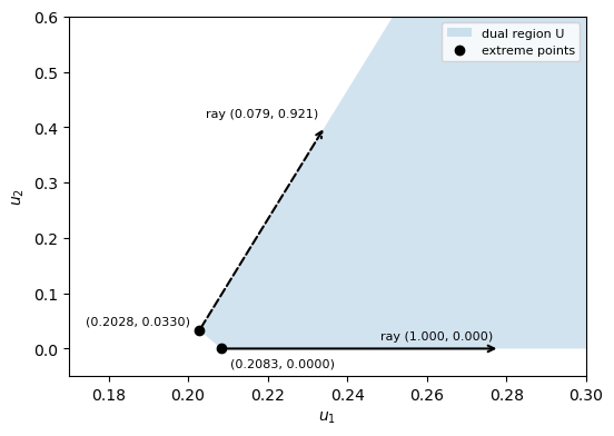

The dual region is an unbounded wedge with two corners close together, (0.2028, 0.0330) and (0.2083, 0); one ray runs right along the u1 axis from (0.2083, 0) and the other climbs steeply along the region's left edge, in direction (0.079, 0.921), from (0.2028, 0.0330).

For fixed $x$ , the $y$ -problem's best value is the dual's minimum of $r_1 u_1 + r_2 u_2$ over $U$ , where $r_1 = 80 - 9x_1 - 4x_2 - 14x_3$ and $r_2 = 10 + x_1 + 2x_2 - 3x_3$ . A linear function's minimum over $U$ sits at a corner, unless it falls forever along a ray. So the whole problem is

\begin{aligned} \max\ 2x_1 + x_2 + 13x_3 + z \quad \text{s.t.}\quad z &\le r_1 p_1 + r_2 p_2 \ \text{ for each corner } p \\ 0 &\le r_1 d_1 + r_2 d_2 \ \text{ for each ray } d, \end{aligned}

with no $y$ at all: two optimality cuts and two feasibility cuts. Predict: does this four-row model give the same optimum as the original?

allcuts = gp.Model("all_cuts")
allcuts.Params.OutputFlag = 0
x = allcuts.addVars(3, vtype=GRB.INTEGER, name="x")
z = allcuts.addVar(lb=-GRB.INFINITY, name="z")
r1 = 80 - 9 * x[0] - 4 * x[1] - 14 * x[2]
r2 = 10 + x[0] + 2 * x[1] - 3 * x[2]
for p in corners:
    allcuts.addConstr(z <= r1 * p[0] + r2 * p[1])
for d in rays:
    allcuts.addConstr(r1 * d[0] + r2 * d[1] >= 0)
allcuts.setObjective(2 * x[0] + x[1] + 13 * x[2] + z, GRB.MAXIMIZE)
allcuts.optimize()
print(f"all-cuts master: value = {allcuts.ObjVal:g}, x = {[round(x[i].X) for i in range(3)]}, z = {z.X:g}")

Restricted license - for non-production use only - expires 2027-11-29
all-cuts master: value = 58, x = [0, 6, 4], z = 0

And the original model, solved in one piece:

orig = gp.Model("original")
orig.Params.OutputFlag = 0
xo = orig.addVars(3, vtype=GRB.INTEGER, name="x")
yo = orig.addVars(2, name="y")
orig.addConstr(9 * xo[0] + 4 * xo[1] + 14 * xo[2] + 35 * yo[0] + 24 * yo[1] <= 80)
orig.addConstr(-xo[0] - 2 * xo[1] + 3 * xo[2] - 3 * yo[0] + 4 * yo[1] <= 10)
orig.setObjective(2 * xo[0] + xo[1] + 13 * xo[2] + 7 * yo[0] + 5 * yo[1], GRB.MAXIMIZE)
orig.optimize()
print(f"original:        value = {orig.ObjVal:g}, x = {[round(xo[i].X) for i in range(3)]}")

original:        value = 58, x = [0, 6, 4]

Here $U$ has two corners and two rays, so writing every cut down is easy. A larger $U$ can have more corners than anyone could list. Benders generates the rows only as the master needs them. Dantzig-Wolfe turns the same idea sideways: write a set of primal variables as a combination of the corners of their feasible set, give each corner a variable (a column), and generate the columns only as they are needed. That is column generation.

Column generation: the cutting stock problem

Rods are 218 cm long. Customers need 44 pieces of 81 cm, 3 pieces of 70 cm and 48 pieces of 68 cm. A pattern $a = (a_1, a_2, a_3)$ says how many pieces of each length one rod is cut into; it fits when $81a_1 + 70a_2 + 68a_3 \le 218$ . With $\lambda_p$ rods cut by pattern $p$ , the master problem is

\min\ \sum_p \lambda_p \quad \text{s.t.}\quad \sum_p a_{ip}\lambda_p \ge d_i \ \text{ for each length } i,\quad \lambda \ge 0 .

Start with three wasteful patterns: one piece per rod.

w = np.array([81, 70, 68])
demand = np.array([44, 3, 48])
L = 218
patterns = [[1, 0, 0], [0, 1, 0], [0, 0, 1]]
print("lengths", w, "| demand", demand, "| start patterns", patterns)

lengths [81 70 68] | demand [44  3 48] | start patterns [[1, 0, 0], [0, 1, 0], [0, 0, 1]]

The restricted master LP

"Restricted" because it holds only the patterns found so far. Its duals $\pi_i$ price one piece of each length. Predict the number of rods and the three duals.

master = gp.Model("master")
master.Params.OutputFlag = 0
lam = [master.addVar(obj=1) for p in patterns]
rows = [master.addConstr(gp.quicksum(p[i] * lam[j] for j, p in enumerate(patterns)) >= demand[i])
        for i in range(3)]
master.optimize()
pi = [con.Pi for con in rows]
print(f"rods = {master.ObjVal:g}, duals = {np.round(pi, 4)}")

rods = 95, duals = [1. 1. 1.]

Pricing: a knapsack problem

A new pattern $a$ costs one rod and is worth $\pi^\top a$ at today's prices, so its reduced cost is $1 - \pi^\top a$ . The pattern with the most negative reduced cost solves a knapsack problem: $\max\ \pi^\top a$ subject to $81a_1 + 70a_2 + 68a_3 \le 218$ , $a$ integer. Predict the pattern.

knap = gp.Model("pricing")
knap.Params.OutputFlag = 0
a = knap.addVars(3, vtype=GRB.INTEGER, name="a")
knap.addConstr(gp.quicksum(w[i] * a[i] for i in range(3)) <= L)
knap.setObjective(gp.quicksum(pi[i] * a[i] for i in range(3)), GRB.MAXIMIZE)
knap.optimize()
new = [round(a[i].X) for i in range(3)]
print(f"new pattern = {new}, uses {w @ new} cm, reduced cost = {1 - knap.ObjVal:g}")

new pattern = [0, 0, 3], uses 204 cm, reduced cost = -2

Add the column

The new pattern becomes a new variable, entering each demand row with its piece count. Predict the new number of rods.

patterns.append(new)
lam.append(master.addVar(obj=1, column=gp.Column(new, rows)))
master.optimize()
pi = [con.Pi for con in rows]
print(f"rods = {master.ObjVal:g}, duals = {np.round(pi, 4)}")

rods = 63, duals = [1.     1.     0.3333]

Now the streamlined version

One round is solve, price, add. The loop repeats it until no pattern has a negative reduced cost. It starts again from the three one-piece patterns, so its first line should match the round above.

patterns = [[1, 0, 0], [0, 1, 0], [0, 0, 1]]
master = gp.Model("master")
master.Params.OutputFlag = 0
lam = [master.addVar(obj=1) for p in patterns]
rows = [master.addConstr(gp.quicksum(p[i] * lam[j] for j, p in enumerate(patterns)) >= demand[i])
        for i in range(3)]
for it in range(1, 50):
    master.optimize()
    pi = [con.Pi for con in rows]
    knap.setObjective(gp.quicksum(pi[i] * a[i] for i in range(3)), GRB.MAXIMIZE)
    knap.optimize()
    new = [round(a[i].X) for i in range(3)]
    rc = 1 - knap.ObjVal
    print(f"round {it}: rods (LP) = {master.ObjVal:5.2f}  duals = {np.round(pi, 3)}  best pattern = {new}  reduced cost = {rc:.3f}")
    if rc > -1e-9:
        break
    patterns.append(new)
    lam.append(master.addVar(obj=1, column=gp.Column(new, rows)))

round 1: rods (LP) = 95.00  duals = [1. 1. 1.]  best pattern = [0, 0, 3]  reduced cost = -2.000
round 2: rods (LP) = 63.00  duals = [1.    1.    0.333]  best pattern = [0, 3, 0]  reduced cost = -2.000
round 3: rods (LP) = 61.00  duals = [1.    0.333 0.333]  best pattern = [2, 0, 0]  reduced cost = -1.000
round 4: rods (LP) = 39.00  duals = [0.5   0.333 0.333]  best pattern = [1, 0, 2]  reduced cost = -0.167
round 5: rods (LP) = 35.00  duals = [0.5   0.333 0.25 ]  best pattern = [2, 0, 0]  reduced cost = 0.000

The patterns the master ended with, and how many rods it cuts by each.

table = pd.DataFrame(patterns, columns=["81 cm", "70 cm", "68 cm"])
table["cm used"] = table[["81 cm", "70 cm", "68 cm"]].values @ w
table["rods (LP)"] = [round(v.X, 3) for v in lam]
table

	81 cm	70 cm	68 cm	cm used	rods (LP)
0	1	0	0	81	0.0
1	0	1	0	70	0.0
2	0	0	1	68	0.0
3	0	0	3	204	0.0
4	0	3	0	210	1.0
5	2	0	0	162	10.0
6	1	0	2	217	24.0

An integer solution from the final master

Rods come whole. Make every $\lambda_p$ integer and re-solve the master over the same patterns. Predict: how many rods, compared with the LP's?

for v in lam:
    v.VType = GRB.INTEGER
master.optimize()
print(f"rods (integer) = {master.ObjVal:g}, by pattern = {[round(v.X) for v in lam]}")

rods (integer) = 35, by pattern = [0, 0, 0, 0, 1, 10, 24]

Column generation never looked at most patterns. This problem is small enough to list them all, so check: solve the integer master with every pattern that fits. Predict how many patterns there are.

every = [p for p in itertools.product(range(3), range(4), range(4)) if 0 < w @ p <= L]
check = gp.Model("every_pattern")
check.Params.OutputFlag = 0
mu = check.addVars(len(every), vtype=GRB.INTEGER)
for i in range(3):
    check.addConstr(gp.quicksum(p[i] * mu[j] for j, p in enumerate(every)) >= demand[i])
check.setObjective(mu.sum(), GRB.MINIMIZE)
check.optimize()
print(f"{len(every)} patterns fit | rods (integer, every pattern) = {check.ObjVal:g}")

14 patterns fit | rods (integer, every pattern) = 35

Compare the LP's rods by pattern with the integer ones. When could an integer master over only the generated patterns miss a better solution that needs a pattern it never generated?
The last round's best pattern was already in the master. Why does that mean the LP is optimal over all patterns, not just the ones generated?
In the all-cuts model, one corner of $U$ never decided the answer. Which one, and how would Benders have found that out?

Going further: the integer programming notebooks in the lab's teaching library.