GurobiPy Beyond LP: Quadratic Constraints, Piecewise-Linear Functions and Multiple Objectives

Teaching · IE 3315 Operations Research I

Python, run with the free Gurobi licence where it uses Gurobi. Download the notebook to run it yourself. First published January 6, 2020 (in R).

Gurobi is not only an LP and MIP solver. This page builds four small models that step past straight lines: a quadratic objective, quadratic constraints, a curved objective approximated by straight pieces, and a model with several objectives ranked by priority. Each is written the same way as an LP; what changes is what the solver has to do with it.

To run it yourself: pip install gurobipy numpy pandas matplotlib. The free licence that comes with pip install gurobipy is enough for everything here.

import numpy as np
import pandas as pd
import matplotlib.pyplot as plt
import gurobipy as gp
from gurobipy import GRB

A quadratic objective

\begin{aligned} \min\ & x^2 + xy + y^2 + yz + z^2 + 2x \\ \text{s.t.}\ & x + 2y + 3z \ge 4 \\ & x + y \ge 1 \\ & x,\ y,\ z \ge 0 \end{aligned}

Products of variables are typed as products. Gurobi sees the objective is quadratic and treats the model as a QP.

qp = gp.Model("qp")
qp.Params.OutputFlag = 0
x, y, z = [qp.addVar(name=n) for n in "xyz"]
qp.setObjective(x * x + x * y + y * y + y * z + z * z + 2 * x, GRB.MINIMIZE)
qp.addConstr(x + 2 * y + 3 * z >= 4)
qp.addConstr(x + y >= 1)
qp.update()
print("IsQP =", qp.IsQP)

Restricted license - for non-production use only - expires 2027-11-29
IsQP = 1

Predict: the $2x$ term makes $x$ costly. Will $x$ be zero at the optimum?

qp.optimize()
print(f"objective = {qp.ObjVal:.4f} | x, y, z = {x.X:.4f}, {y.X:.4f}, {z.X:.4f}")

objective = 2.1111 | x, y, z = 0.0000, 1.0000, 0.6667

Now require whole numbers. Changing each variable's VType turns the QP into a mixed-integer QP. Predict: can the objective go down?

for v in (x, y, z):
    v.VType = GRB.INTEGER
qp.optimize()
print(f"objective = {qp.ObjVal:.4f} | x, y, z = {x.X:.0f}, {y.X:.0f}, {z.X:.0f}")

objective = 3.0000 | x, y, z = 0, 1, 1

Quadratic constraints: two cones

\begin{aligned} \max\ & x \\ \text{s.t.}\ & x + y + z = 1 \\ & x^2 + y^2 \le z^2 \\ & x^2 \le yz \\ & x,\ y,\ z \ge 0 \end{aligned}

With $z \ge 0$ , $x^2 + y^2 \le z^2$ says the point $(x, y)$ lies within distance $z$ of the origin: a second-order cone. $x^2 \le yz$ with $y, z \ge 0$ is a rotated cone. Both regions are convex, even though $-z^2$ and $-yz$ look like trouble on their own.

qc = gp.Model("qcp")
qc.Params.OutputFlag = 0
x, y, z = [qc.addVar(name=n) for n in "xyz"]
qc.setObjective(x, GRB.MAXIMIZE)
qc.addConstr(x + y + z == 1, name="sum")
cone = qc.addConstr(x * x + y * y - z * z <= 0, name="cone")
rotated = qc.addConstr(x * x - y * z <= 0, name="rotated_cone")
qc.update()
print(qc.NumConstrs, "linear constraint,", qc.NumQConstrs, "quadratic constraints")

1 linear constraint, 2 quadratic constraints

Predict: $x$ has to share a total of 1 with $y$ and $z$ . Can it reach $\tfrac{1}{2}$ ?

qc.optimize()
print(f"x = {x.X:.4f}, y = {y.X:.4f}, z = {z.X:.4f} | IsMIP = {qc.IsMIP}")

x = 0.3270, y = 0.2571, z = 0.4159 | IsMIP = 0

When a quadratic constraint is not convex

Flip the first cone to $x^2 + y^2 \ge z^2$ . The points outside a cone do not form a convex set, so the solver can no longer rely on any local optimum being the best one. Before version 11, Gurobi stopped with an error here unless you set the parameter NonConvex = 2. Setting it to 1 brings that behaviour back:

qc.remove(cone)
qc.addConstr(x * x + y * y - z * z >= 0, name="outside_cone")
qc.Params.NonConvex = 1
try:
    qc.optimize()
except gp.GurobiError as err:
    print("error", err.errno, ":", err)

error 10020 : Constraint Q not PSD (negative diagonal entry). Set NonConvex parameter to -1 or 2 to solve model.

Back to the default (-1), which in current Gurobi accepts non-convex quadratics and searches for the global optimum by branching, the way it does for a MIP. Predict: is the new optimum above or below the cone answer?

qc.Params.NonConvex = -1
qc.optimize()
print(f"x = {x.X:.4f}, y = {y.X:.4f}, z = {z.X:.4f} | IsMIP = {qc.IsMIP}")

x = 0.3333, y = 0.3333, z = 0.3333 | IsMIP = 1

Piecewise-linear objectives

\begin{aligned} \min\ & f(x) - y + g(z) \\ \text{s.t.}\ & x + 2y + 3z \le 4 \\ & x + y \ge 1 \\ & 0 \le x,\ y,\ z \le 1 \end{aligned} \qquad \begin{aligned} f(x) &= e^{-x} \\ g(z) &= 2z^2 - 4z \end{aligned}

Instead of the curves, give Gurobi points on them. It joins the points with straight segments, so the objective becomes piecewise linear. Here are 101 points between 0 and 1.

u = np.linspace(0, 1, 101)
f = np.exp(-u)
g = 2 * u**2 - 4 * u
print(len(u), "breakpoints | f from", f[0], "to", round(f[-1], 4), "| g from", g[0], "to", g[-1])

101 breakpoints | f from 1.0 to 0.3679 | g from 0.0 to -2.0

The two functions, and the negation of $f$ that comes next. A minimisation with a convex piecewise-linear objective is still an LP; with a concave piece, it is not.

fig, ax = plt.subplots(figsize=(6, 4.2))
ax.plot(u, f, label=r"$f(x) = e^{-x}$ (convex)")
ax.plot(u, -f, "--", label=r"$-f(x) = -e^{-x}$ (concave)")
ax.plot(u, g, "-.", label=r"$g(z) = 2z^2 - 4z$ (convex)")
ax.set(xlabel="value of the variable, 0 to 1", ylabel="function value")
ax.legend(fontsize=8)
plt.show()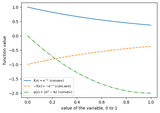

$On 0 to 1, e^{-x} falls from 1 to 0.37 bending upward, its negation rises from -1 to -0.37 bending downward, and 2z^2 - 4z falls from 0 to -2 bending upward.$

setPWLObj attaches a piecewise-linear objective term to one variable; the linear $-y$ goes in the ordinary Obj attribute.

pw = gp.Model("pwl")
pw.Params.OutputFlag = 0
x, y, z = [pw.addVar(ub=1, name=n) for n in "xyz"]
pw.addConstr(x + 2 * y + 3 * z <= 4)
pw.addConstr(x + y >= 1)
y.Obj = -1
pw.setPWLObj(x, u, f)
pw.setPWLObj(z, u, g)
pw.update()
print(pw.NumVars, "variables,", pw.NumConstrs, "constraints, minimise")

3 variables, 2 constraints, minimise

Predict: $f$ falls as $x$ grows and $g$ falls as $z$ grows, but the first constraint caps them. Where do $x$ , $y$ and $z$ land?

pw.optimize()
print(f"objective = {pw.ObjVal:.4f} | x, y, z = {x.X:.4f}, {y.X:.4f}, {z.X:.4f} | IsMIP = {pw.IsMIP}")

objective = -1.9346 | x, y, z = 0.6900, 0.7250, 0.6200 | IsMIP = 0

Now replace $f$ with $-f$ , the concave curve in the figure. Predict: does the solution move, and does Gurobi still solve it as an LP?

pw.setPWLObj(x, u, -f)
pw.optimize()
print(f"objective = {pw.ObjVal:.4f} | x, y, z = {x.X:.4f}, {y.X:.4f}, {z.X:.4f} | IsMIP = {pw.IsMIP}")

objective = -3.7777 | x, y, z = 0.0000, 1.0000, 0.6667 | IsMIP = 1

Multiple objectives, ranked

Twenty elements; pick at most 12. Four sets each want as many of their own elements picked as possible. The sets do not matter equally: set 1 has the highest priority, sets 2 and 3 share the next, set 4 comes last.

sets = np.array([
    [1, 1, 1, 1, 1, 1, 1, 1, 1, 1, 0, 0, 0, 0, 0, 0, 0, 0, 0, 0],
    [0, 0, 0, 0, 0, 1, 1, 1, 1, 1, 0, 0, 0, 0, 0, 1, 1, 1, 1, 1],
    [0, 0, 0, 1, 1, 0, 1, 1, 0, 0, 0, 0, 0, 1, 1, 0, 1, 1, 0, 0],
    [0, 0, 0, 1, 1, 1, 0, 0, 0, 1, 1, 1, 0, 0, 0, 1, 1, 1, 0, 0]])
priority = [3, 2, 2, 1]
weight = [1.0, 0.25, 1.25, 1.0]
print("elements in each set:", sets.sum(axis=1), "| budget: 12")

elements in each set: [10 10  8  9] | budget: 12

setObjectiveN adds one objective at a time. Gurobi optimises the highest priority first, then the next while holding the first near its best. "Near" is set by abstol and reltol: how much each objective may give up for the ones below it. Objectives with the same priority are added together using their weights.

mo = gp.Model("multiobj")
mo.Params.OutputFlag = 0
pick = mo.addMVar(20, vtype=GRB.BINARY, name="pick")
mo.addConstr(pick.sum() <= 12, name="budget")
mo.ModelSense = GRB.MAXIMIZE
for i in range(4):
    mo.setObjectiveN(sets[i] @ pick, index=i, priority=priority[i], weight=weight[i],
                     abstol=i + 1, reltol=0.01, name=f"set{i + 1}")
mo.update()
print(mo.NumObj, "objectives,", mo.NumVars, "binary variables")

4 objectives, 20 binary variables

Predict: set 1 has 10 elements and the budget is 12. How many of set 1's elements will be picked? PoolSolutions asks Gurobi to keep up to 100 of the solutions it finds, not just the best.

mo.Params.PoolSolutions = 100
mo.optimize()
print("picked elements:", [e + 1 for e in range(20) if pick.X[e] > 0.5])
for i in range(4):
    mo.Params.ObjNumber = i
    print(f"set{i + 1}: {mo.ObjNVal:.0f} of {sets[i].sum()} covered")

picked elements: [2, 3, 4, 5, 6, 7, 8, 9, 10, 11, 12, 17]
set1: 9 of 10 covered
set2: 6 of 10 covered
set3: 5 of 8 covered
set4: 7 of 9 covered

The solution pool

Each pooled solution is read by setting SolutionNumber; ObjNVal then gives that solution's value of the objective chosen by ObjNumber. Here are up to the first 10.

print("solutions in the pool:", mo.SolCount)
rows = []
for k in range(min(10, mo.SolCount)):
    mo.Params.SolutionNumber = k
    row = {}
    for i in range(4):
        mo.Params.ObjNumber = i
        row[f"set{i + 1}"] = mo.ObjNVal
    rows.append(row)
pd.DataFrame(rows).astype(int)

solutions in the pool: 3

	set1	set2	set3	set4
0	9	6	5	7
1	9	7	7	6
2	10	5	4	4

Questions to try:

In the QP, requiring whole numbers raised the minimum. Could adding integer requirements ever lower it?
In the piecewise-linear model, why does a concave piece force Gurobi to add binary variables, while a convex one does not?
Row 2 of the pool covers all 10 elements of set 1, yet Gurobi returned a solution covering 9. Which setting allowed that? Change it for set 1 and re-solve.

Going further: the nonlinear and convex notebooks in the lab's teaching library.