Light Rail in a Model City

May 3, 2019 · Systems Modeling

Background

I extended the work of (Wu and Plantinga 2003) using R and certain equation modififications to investigate how the addition of a light rail line would influence a city.

Cities have housed most of the human race since 2004 and as a result influence most of the individual, commercial, and industrial energy and GHG patterns. However, city designs, have placed amenities in isolated suburban pockets, the abundance of roads have encouraged sprawl, and zoning laws have discouraged density. Therefore, for this study I will investigate how these choices can positively or negatively influence a city’s environmental footprint.

I extended the work of (Wu and Plantinga 2003) using R and certain equation modififications to investigate how the addition of a light rail line would influence a city. First, I tried to replicate their city without any parks using their parameters. Second, I made some modifications to get the city to a scale that I could represent graphically. Third, I modeled the light rail as an amenity to see the influence it has on the city. Finally, I modeled the light rail so that it reduced travel costs for the citizens close to it instead of providing an amenity value. The parameters I used where nearly identical to the (Wu and Plantinga 2003) parameters; however I did have to make some minor modifications. The given utility produced a much larger area then was graphically tractable, so I increased it to 6,000 for all the models excluding the original monocentric model which uses the original utility value. The transport cost for the rail is set to half of the normal transport costs (t¬¬rail=$500). The original parameters are shown in Table 1.

Wu, Jun Jie, and Andrew J. Plantinga. 2003. “The Influence of Public Open Space on Urban Spatial Structure.” Journal of Environmental Economics and Management 46 (2): 288–309. https://doi.org/10.1016/S0095-0696(03)00023-8.

require(ggplot2)

## Loading required package: ggplot2

## Warning: package 'ggplot2' was built under R version 4.1.2

require(grid)

## Loading required package: grid

require(gridExtra)

## Loading required package: gridExtra

## Warning: package 'gridExtra' was built under R version 4.1.2

require(RColorBrewer)

## Loading required package: RColorBrewer

require(viridis)

## Loading required package: viridis

## Warning: package 'viridis' was built under R version 4.1.2

## Loading required package: viridisLite

## Warning: package 'viridisLite' was built under R version 4.1.2

Parameters

#budget 
#median income per capita Austin https://www.deptofnumbers.com/income/texas/austin/
y <- 40000

u <- c(0:150)
v <- c(0:150)

#Loop to give 15 miles worth of u and v

i <- 0
j <- 0
ii <- 1

while(i < 151){
  
  j <- 0
  while(j < 151){
  u[ii] <- i/5 - 15
  v[ii] <- j/5 - 15
  j <- j+1
  ii <- ii+1
  }
  
  i <- i +1
  
}

#distance from center
x <- sqrt(u^2+v^2)

#transportation cost 50 cents a mile by 320 days
t <- 1000
#housing price per sqft vector
p <- c(0:150)
#housing consumption (sqft) by mile vector
q <- c(0:150)
#general good
g <- c(0:150)
#utility level
V <- 4200
#alpha for Cobb Douglas
al <- .5
#beta for development cobb-douglas
bt <- 4/3
#capital 
c0 <- 0

#amentiy
ad <- 0.16
ng <- 1
d <- 0

#gamma for amenity
gm <- 0.5

#z distance to amentiy
z <- sqrt((x-d)^2)

#land rent/acre
r <- c(0:150)
#Housing floor space / acre
s <- c(0:150)
#ag rent
#Ausitn is about 8000 https://heritagelandbank.com/announcements/news-events/how-much-average-price-land-texas
ag <- 8000


#Multiplier values
tm1 <- 1 - 0
tm2 <- 1 - 0
tm3 <- 1 - 0
tm4 <- 1 - 0

im1 <- 1 + 0
im2 <- 1 + 0
im3 <- 1 + 0
im4 <- 1 + 0

am1 <- 1 + 0
am2 <- 1 + 0
am3 <- 1 + 0
am4 <- 1 + 0

Monocentric original model parameters

Iterations to determine Utility Value (V) that gives start of about 100k

V <- 4000

i <- 1

NN <- c(1:10)

while(i <= 10){

#finding x for various u,v
x <- sqrt(u^2+v^2)

#z distance to amentiy
z <- sqrt((x-d)^2)

#amentiy distribution
am <- 1 + ad*(exp(-ng*z))

#finding the price for various u,v
p <- (al^al*(1-al)^(1-al)*am^gm*(y-t*x)/V)^(1/al)

#optimal q
q <- al*(y-t*x)/p

#optimal g
g <- (1-al)*(y-t*x)



#theta some funciton of beta
ph <- ((bt-1)^((bt-1)/bt))/bt

#optimal r

r <- (ph*p)^(bt/(bt-1))

r1 <- ((ph*al)^al * (1-al)^(1-al) * (y-t*x)/V)^(bt/(al*(bt-1)))

#optimal s
s <- (p/bt)^(1/(bt-1))

s1 <- (bt-1)^(-1/bt) * (r)^(1/bt)




#population n s(floorspaceperacre/ floorspace per household * (size of square (sqmi)) * acres/sqmi * fraction of housing in area)
n <- s/q * (.2*.2) * 640 * .25  
#s <- n*q /(1 * 640 * .25 )
#q <-  s/(n*(1 * 640 * .25 ))



#Utility Value

U <- q^al*g^(1-al)

dfsc <- data.frame(u,v,x,p,g,q,s,r,U,n)

#delete values where ag rent exceeds land rent
dfsc1 <- dfsc[(dfsc$r > ag),]

#total population
NN[i] <- sum(dfsc1$n)

print(V)

V <- V + 50

i <- i + 1



}

## [1] 4000
## [1] 4050
## [1] 4100
## [1] 4150
## [1] 4200
## [1] 4250
## [1] 4300
## [1] 4350
## [1] 4400
## [1] 4450

dfsc1

##          u    v         x        p        g         q        s         r
## 8531  -3.8 -0.2 3.8052595 16.59795 18097.37 1090.3376 1929.067  8004.640
## 8532  -3.8  0.0 3.8000000 16.60309 18100.00 1090.1587 1930.858  8014.550
## 8533  -3.8  0.2 3.8052595 16.59795 18097.37 1090.3376 1929.067  8004.640
## 8677  -3.6 -1.2 3.7947332 16.60823 18102.63 1089.9796 1932.653  8024.487
## 8678  -3.6 -1.0 3.7363083 16.66547 18131.85 1087.9889 1952.704  8135.684
## 8679  -3.6 -0.8 3.6878178 16.71322 18156.09 1086.3309 1969.539  8229.335
## 8680  -3.6 -0.6 3.6496575 16.75097 18175.17 1085.0221 1982.913  8303.926
## 8681  -3.6 -0.4 3.6221541 16.77826 18188.92 1084.0766 1992.622  8358.184
## 8682  -3.6 -0.2 3.6055513 16.79478 18197.22 1083.5048 1998.512  8391.142
## 8683  -3.6  0.0 3.6000000 16.80031 18200.00 1083.3134 2000.486  8402.197
## 8684  -3.6  0.2 3.6055513 16.79478 18197.22 1083.5048 1998.512  8391.142
## … 2,260 more rows not shown …
## 14125 4442.015 11.34790
## 14269 4442.099 11.32312
## 14270 4442.057 11.33550
## 14271 4442.099 11.32312

nrow(dfsc1$n)

## NULL

sum(dfsc1$n)

## [1] 17997.98

NN

##  [1] 99500.53 84673.14 71395.90 60045.24 50182.63 41877.02 34273.63 27997.58
##  [9] 22468.26 17997.98

#Reseting Parameters for All Cities


V <- 4000
#housing price per sqft vector
p <- c(0:150)
#housing consumption (sqft) by mile vector
q <- c(0:150)
#general good
g <- c(0:150)

#land rent/acre
r <- c(0:150)
#Housing floor space / acre
s <- c(0:150)

City 1

New t,y,and ad multiplication factors

t <- 1000*tm1

y <- 40000*im1

ad <- 0.16*am1



#finding x for various u,v
x <- sqrt(u^2+v^2)

#finding distance to rail
z <- sqrt((x-d)^2)


#amentiy distribution
am <- 1 + ad*(exp(-ng*z))

#finding the price for various u,v
p <- (al^al*(1-al)^(1-al)*am^gm*(y-t*x)/V)^(1/al)

#optimal q
q <- al*(y-t*x)/p

#optimal g
g <- (1-al)*(y-t*x)


#theta some funciton of beta
ph <- ((bt-1)^((bt-1)/bt))/bt

#optimal r

r <- (ph*p)^(bt/(bt-1))

r1 <- ((ph*al)^al * (1-al)^(1-al) * (y-t*x)/V)^(bt/(al*(bt-1)))

#optimal s
s <- (p/bt)^(1/(bt-1))

s1 <- (bt-1)^(-1/bt) * (r)^(1/bt)

#Utility Value

U <- q^al*g^(1-al)


#population n s(floorspaceperacre/ floorspace per household * (size of square (sqmi)) * acres/sqmi * fraction of housing in area)
n <- s/q * (.2*.2) * 640 * .25 

nn <- s/q



dfscm <- data.frame(u,v,t,x,p,g,q,s,r,U,n,nn)

#delete values where ag rent exceeds land rent
dfscm1 <- dfscm[(dfscm$r > ag),]

head(dfscm1)

##         u    v    t        x        p        g        q        s        r
## 5812 -7.4 -0.4 1000 7.410803 16.59623 16294.60 981.8255 1928.466 8001.313
## 5813 -7.4 -0.2 1000 7.402702 16.60449 16298.65 981.5807 1931.348 8017.263
## 5814 -7.4  0.0 1000 7.400000 16.60725 16300.00 981.4991 1932.310 8022.590
## 5815 -7.4  0.2 1000 7.402702 16.60449 16298.65 981.5807 1931.348 8017.263
## 5816 -7.4  0.4 1000 7.410803 16.59623 16294.60 981.8255 1928.466 8001.313
## 5957 -7.2 -1.6 1000 7.375636 16.63212 16312.18 980.7637 1941.006 8070.760
##             U        n       nn
## 5812 3999.807 12.57064 1.964163
## 5813 3999.805 12.59257 1.967590
## 5814 3999.804 12.59990 1.968734
## 5815 3999.805 12.59257 1.967590
## 5816 3999.807 12.57064 1.964163
## 5957 3999.800 12.66608 1.979076

#Total Land Area of the City

print('Land Area')

## [1] "Land Area"

nrow(dfscm1)*(.2*.2)

## [1] 172.68

max(dfscm1$u)

## [1] 7.4

max(dfscm1$v)

## [1] 7.4

#Total Population

print('Population')

## [1] "Population"

round(sum(dfscm1$n),0)

## [1] 99501

p1<-ggplot(dfscm1, aes(x = u, y = v, color = n)) +
   geom_point(size = 2, shape = 7) +
  
  scale_color_viridis(limits = c(5,150), direction = -1) +
  lims(x=c(-15,15),y=c(-15,15)) +
  coord_fixed() +  
  theme_minimal()+
  geom_vline(xintercept = 0) + 
  geom_hline(yintercept = 0) +
  labs(title = 'City 1')

City 2

New t,y,and ad multiplication factors

t <- 1000*tm2

y <- 40000*im2

ad <- 0.16*am2


#finding x for various u,v
x <- sqrt(u^2+v^2)

#finding distance to rail
z <- sqrt((x-d)^2)


#amentiy distribution
am <- 1 + ad*(exp(-ng*z))

#finding the price for various u,v
p <- (al^al*(1-al)^(1-al)*am^gm*(y-t*x)/V)^(1/al)

#optimal q
q <- al*(y-t*x)/p

#optimal g
g <- (1-al)*(y-t*x)


#theta some funciton of beta
ph <- ((bt-1)^((bt-1)/bt))/bt

#optimal r

r <- (ph*p)^(bt/(bt-1))

r1 <- ((ph*al)^al * (1-al)^(1-al) * (y-t*x)/V)^(bt/(al*(bt-1)))

#optimal s
s <- (p/bt)^(1/(bt-1))

s1 <- (bt-1)^(-1/bt) * (r)^(1/bt)

#Utility Value

U <- q^al*g^(1-al)


#population n s(floorspaceperacre/ floorspace per household * (size of square (sqmi)) * acres/sqmi * fraction of housing in area)
n <- s/q * (.2*.2) * 640 * .25 

nn <- s/q



dfscm <- data.frame(u,v,t,x,p,g,q,s,r,U,n,nn)

#delete values where ag rent exceeds land rent
dfscm2 <- dfscm[(dfscm$r > ag),]

head(dfscm2)

##         u    v    t        x        p        g        q        s        r
## 5812 -7.4 -0.4 1000 7.410803 16.59623 16294.60 981.8255 1928.466 8001.313
## 5813 -7.4 -0.2 1000 7.402702 16.60449 16298.65 981.5807 1931.348 8017.263
## 5814 -7.4  0.0 1000 7.400000 16.60725 16300.00 981.4991 1932.310 8022.590
## 5815 -7.4  0.2 1000 7.402702 16.60449 16298.65 981.5807 1931.348 8017.263
## 5816 -7.4  0.4 1000 7.410803 16.59623 16294.60 981.8255 1928.466 8001.313
## 5957 -7.2 -1.6 1000 7.375636 16.63212 16312.18 980.7637 1941.006 8070.760
##             U        n       nn
## 5812 3999.807 12.57064 1.964163
## 5813 3999.805 12.59257 1.967590
## 5814 3999.804 12.59990 1.968734
## 5815 3999.805 12.59257 1.967590
## 5816 3999.807 12.57064 1.964163
## 5957 3999.800 12.66608 1.979076

#Total Land Area of the City

print('Land Area')

## [1] "Land Area"

nrow(dfscm2)*(.2*.2)

## [1] 172.68

max(dfscm2$u)

## [1] 7.4

max(dfscm2$v)

## [1] 7.4

#Total Population

print('Population')

## [1] "Population"

round(sum(dfscm2$n),0)

## [1] 99501

p2<-ggplot(dfscm2, aes(x = u, y = v, color = n)) +
   geom_point(size = 2, shape = 7) +
  
  scale_color_viridis(limits = c(5,150), direction = -1) +
  lims(x=c(-15,15),y=c(-15,15)) +
  coord_fixed() +  
  theme_minimal()+
  geom_vline(xintercept = 0) + 
  geom_hline(yintercept = 0) +
  labs(title = 'City 2')

City 3

New t,y,and ad multiplication factors

t <- 1000*tm3

y <- 40000*im3

ad <- 0.16*am3


#finding x for various u,v
x <- sqrt(u^2+v^2)

#finding distance to rail
z <- sqrt((x-d)^2)


#amentiy distribution
am <- 1 + ad*(exp(-ng*z))

#finding the price for various u,v
p <- (al^al*(1-al)^(1-al)*am^gm*(y-t*x)/V)^(1/al)

#optimal q
q <- al*(y-t*x)/p

#optimal g
g <- (1-al)*(y-t*x)


#theta some funciton of beta
ph <- ((bt-1)^((bt-1)/bt))/bt

#optimal r

r <- (ph*p)^(bt/(bt-1))

r1 <- ((ph*al)^al * (1-al)^(1-al) * (y-t*x)/V)^(bt/(al*(bt-1)))

#optimal s
s <- (p/bt)^(1/(bt-1))

s1 <- (bt-1)^(-1/bt) * (r)^(1/bt)

#Utility Value

U <- q^al*g^(1-al)


#population n s(floorspaceperacre/ floorspace per household * (size of square (sqmi)) * acres/sqmi * fraction of housing in area)
n <- s/q * (.2*.2) * 640 * .25 

nn <- s/q



dfscm <- data.frame(u,v,t,x,p,g,q,s,r,U,n,nn)

#delete values where ag rent exceeds land rent
dfscm3 <- dfscm[(dfscm$r > ag),]

head(dfscm3)

##         u    v    t        x        p        g        q        s        r
## 5812 -7.4 -0.4 1000 7.410803 16.59623 16294.60 981.8255 1928.466 8001.313
## 5813 -7.4 -0.2 1000 7.402702 16.60449 16298.65 981.5807 1931.348 8017.263
## 5814 -7.4  0.0 1000 7.400000 16.60725 16300.00 981.4991 1932.310 8022.590
## 5815 -7.4  0.2 1000 7.402702 16.60449 16298.65 981.5807 1931.348 8017.263
## 5816 -7.4  0.4 1000 7.410803 16.59623 16294.60 981.8255 1928.466 8001.313
## 5957 -7.2 -1.6 1000 7.375636 16.63212 16312.18 980.7637 1941.006 8070.760
##             U        n       nn
## 5812 3999.807 12.57064 1.964163
## 5813 3999.805 12.59257 1.967590
## 5814 3999.804 12.59990 1.968734
## 5815 3999.805 12.59257 1.967590
## 5816 3999.807 12.57064 1.964163
## 5957 3999.800 12.66608 1.979076

#Total Land Area of the City

print('Land Area')

## [1] "Land Area"

nrow(dfscm3)*(.2*.2)

## [1] 172.68

max(dfscm3$u)

## [1] 7.4

max(dfscm3$v)

## [1] 7.4

#Total Population

print('Population')

## [1] "Population"

round(sum(dfscm3$n),0)

## [1] 99501

p3 <- ggplot(dfscm3, aes(x = u, y = v, color = n)) +
   geom_point(size = 2, shape = 7) +
  
  scale_color_viridis(limits = c(5,150), direction = -1) +
  lims(x=c(-15,15),y=c(-15,15)) +
  coord_fixed() +  
  theme_minimal()+
  geom_vline(xintercept = 0) + 
  geom_hline(yintercept = 0) +
  labs(title = 'City 3')

City 4

New t,y,and ad multiplication factors

t <- 1000*tm4

y <- 40000*im4

ad <- 0.16*am4


#finding x for various u,v
x <- sqrt(u^2+v^2)

#finding distance to rail
z <- sqrt((x-d)^2)


#amentiy distribution
am <- 1 + ad*(exp(-ng*z))

#finding the price for various u,v
p <- (al^al*(1-al)^(1-al)*am^gm*(y-t*x)/V)^(1/al)

#optimal q
q <- al*(y-t*x)/p

#optimal g
g <- (1-al)*(y-t*x)


#theta some funciton of beta
ph <- ((bt-1)^((bt-1)/bt))/bt

#optimal r

r <- (ph*p)^(bt/(bt-1))

r1 <- ((ph*al)^al * (1-al)^(1-al) * (y-t*x)/V)^(bt/(al*(bt-1)))

#optimal s
s <- (p/bt)^(1/(bt-1))

s1 <- (bt-1)^(-1/bt) * (r)^(1/bt)

#Utility Value

U <- q^al*g^(1-al)


#population n s(floorspaceperacre/ floorspace per household * (size of square (sqmi)) * acres/sqmi * fraction of housing in area)
n <- s/q * (.2*.2) * 640 * .25 

nn <- s/q



dfscm <- data.frame(u,v,t,x,p,g,q,s,r,U,n,nn)

#delete values where ag rent exceeds land rent
dfscm4 <- dfscm[(dfscm$r > ag),]

head(dfscm4)

##         u    v    t        x        p        g        q        s        r
## 5812 -7.4 -0.4 1000 7.410803 16.59623 16294.60 981.8255 1928.466 8001.313
## 5813 -7.4 -0.2 1000 7.402702 16.60449 16298.65 981.5807 1931.348 8017.263
## 5814 -7.4  0.0 1000 7.400000 16.60725 16300.00 981.4991 1932.310 8022.590
## 5815 -7.4  0.2 1000 7.402702 16.60449 16298.65 981.5807 1931.348 8017.263
## 5816 -7.4  0.4 1000 7.410803 16.59623 16294.60 981.8255 1928.466 8001.313
## 5957 -7.2 -1.6 1000 7.375636 16.63212 16312.18 980.7637 1941.006 8070.760
##             U        n       nn
## 5812 3999.807 12.57064 1.964163
## 5813 3999.805 12.59257 1.967590
## 5814 3999.804 12.59990 1.968734
## 5815 3999.805 12.59257 1.967590
## 5816 3999.807 12.57064 1.964163
## 5957 3999.800 12.66608 1.979076

#Total Land Area of the City

print('Land Area')

## [1] "Land Area"

nrow(dfscm4)*(.2*.2)

## [1] 172.68

max(dfscm4$u)

## [1] 7.4

max(dfscm4$v)

## [1] 7.4

#Total Population

print('Population')

## [1] "Population"

round(sum(dfscm4$n),0)

## [1] 99501

p4 <- ggplot(dfscm4, aes(x = u, y = v, color = n)) +
   geom_point(size = 2, shape = 7) +
  
  scale_color_viridis(limits = c(5,150), direction = -1) +
  lims(x=c(-15,15),y=c(-15,15)) +
  coord_fixed() +  
  theme_minimal()+
  geom_vline(xintercept = 0) + 
  geom_hline(yintercept = 0) +
  labs(title = 'City 4')

Displaying all graphs and Saving All Graphs

#Population Density Across Urban Areas
pop_den <- grid.arrange(p1,p2,p3,p4, ncol=2, nrow = 2)

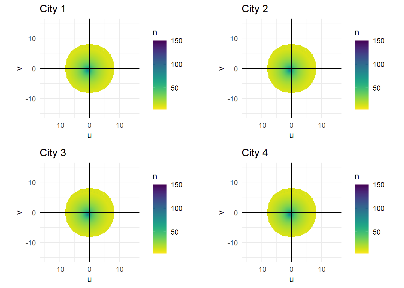
#Land and Population Table

lnda <- c(nrow(dfscm1)*(0.2*0.2),nrow(dfscm2)*(0.2*0.2),nrow(dfscm3)*(0.2*0.2),nrow(dfscm4)*(0.2*0.2))
popg <- c(sum(dfscm1$n),sum(dfscm2$n),sum(dfscm3$n),sum(dfscm4$n))
lap <- data.frame(Land_Area = lnda, Population = round(popg), Population_Density = round(popg/lnda))
rownames(lap) <- c('City 1', 'City 2', 'City 3', 'City 4')
lap

##        Land_Area Population Population_Density
## City 1    172.68      99501                576
## City 2    172.68      99501                576
## City 3    172.68      99501                576
## City 4    172.68      99501                576

# Multiplier Table

mtable <- data.frame(Income_Multiplier = c(im1, im2, im3, im4), Traffic_Multiplier = c(tm1, tm2, tm3, tm4), Amenity_Multiplier = c(am1, am2, am3, am4) )
rownames(mtable) <- c('City 1', 'City 2', 'City 3', 'City 4')
mtable

##        Income_Multiplier Traffic_Multiplier Amenity_Multiplier
## City 1                 1                  1                  1
## City 2                 1                  1                  1
## City 3                 1                  1                  1
## City 4                 1                  1                  1

#Saving files as Pdfs

# pdf("land_pop.pdf", height =2, width = 8.5)
# grid.table(lap)
# dev.off()

# ggsave(filename = "pop_den.pdf", pop_den)