The Basics of Simulation

Teaching · IE 5301 Advanced Operations Research · IE 3301 Engineering Probability

In Python and in R, step by step. Download the Python notebook or the R notebook to run it yourself; a one-page R and Python cheat sheet lists the equivalents. First published January 2, 2020 (in R).

Code:

Every simulation starts from one thing: numbers that look uniformly random on $(0, 1)$ . This page turns those uniforms into coin tosses, binomials, exponentials, Poissons, betas, normals and geometrics, then uses them to simulate a single-server queue and compare it with the textbook formulas, and finishes by estimating areas with random points.

Python and R use different random number generators, so the two versions draw different numbers even from the same seed. The formulas they are checked against are the same.

To run it yourself: pip install numpy pandas matplotlib. Every random number comes from one generator with a fixed seed, so a top-to-bottom run gives the numbers shown here.

To run it yourself you need only base R; there is nothing to install. set.seed(123) fixes the random numbers, so a top-to-bottom run gives the numbers shown here.

Python

import numpy as np
import pandas as pd
import matplotlib.pyplot as plt

rng = np.random.default_rng(123)

set.seed(123)
options(repr.plot.width = 6, repr.plot.height = 4.2, repr.plot.res = 100)

From uniforms to coin tosses

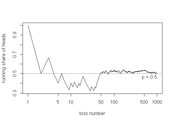
A toss is heads when $U < p$ . With $p = 0.5$ , toss a coin 1,000 times and track the running share of heads. Predict: after how many tosses does the share stay within 0.05 of one half?

Python

U = rng.random(1000)
heads = (U < 0.5).astype(int)
running = heads.cumsum() / np.arange(1, 1001)
fig, ax = plt.subplots(figsize=(6, 4.2))
ax.plot(np.arange(1, 1001), running, label="running share of heads")
ax.axhline(0.5, color="0.3", linestyle="--", label="p = 0.5")
ax.set(xlabel="toss number", ylabel="share of heads", xscale="log")
ax.legend()
plt.show()
outside = np.nonzero(np.abs(running - 0.5) > 0.05)[0]
print("share after 1000 tosses:", running[-1], "| last toss outside 0.45-0.55:", outside[-1] + 1)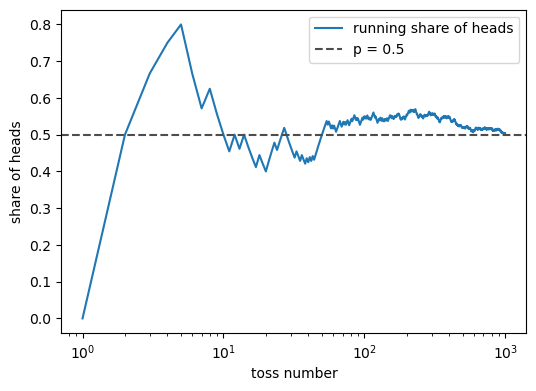

On a log scale of toss number, the running share of heads swings widely over the first few dozen tosses, stays within 0.05 of the dashed line at 0.5 from toss 397 on, and ends at 0.501 after 1,000 tosses.

share after 1000 tosses: 0.501 | last toss outside 0.45-0.55: 396

U <- runif(1000)
heads <- as.integer(U < 0.5)
running <- cumsum(heads) / (1:1000)
plot(1:1000, running, type = "l", log = "x", xlab = "toss number", ylab = "running share of heads")
abline(h = 0.5, col = "gray30", lty = 2)
text(1000, 0.49, "p = 0.5", adj = c(1, 1))    # a text label: legend() boxes come out mis-sized in Jupyter's R kernel
outside <- which(abs(running - 0.5) > 0.05)
cat("share after 1000 tosses:", running[1000], "| last toss outside 0.45-0.55:", max(outside), "\n")

share after 1000 tosses: 0.507 | last toss outside 0.45-0.55: 43

On a log scale of toss number, the running share of heads starts at 1, dips to about 0.32 near toss 30, stays within 0.05 of the dashed line at 0.5 from toss 44 on, and ends at 0.507 after 1,000 tosses.

Each toss is a Bernoulli( $p$ ) variable, and a sum of $n$ of them is Binomial( $n$ , $p$ ). With $n = 1000$ and $p = 0.2$ , do this 5,000 times and compare with the built-in binomial generator. Predict the mean and variance.

Python

X_built = (rng.random((5000, 1000)) < 0.2).sum(axis=1)
X_numpy = rng.binomial(1000, 0.2, size=5000)
print(f"built from uniforms: mean {X_built.mean():.2f}, variance {X_built.var():.1f}")
print(f"numpy's binomial:    mean {X_numpy.mean():.2f}, variance {X_numpy.var():.1f}")
print("formulas: np =", 1000 * 0.2, "| np(1 - p) =", 1000 * 0.2 * 0.8)

built from uniforms: mean 200.29, variance 159.3
numpy's binomial:    mean 200.22, variance 160.9
formulas: np = 200.0 | np(1 - p) = 160.0

X_built <- rowSums(matrix(runif(5000 * 1000) < 0.2, nrow = 5000))
X_rbinom <- rbinom(5000, 1000, 0.2)
cat(sprintf("built from uniforms: mean %.2f, variance %.1f\n", mean(X_built), var(X_built)))
cat(sprintf("R's rbinom:          mean %.2f, variance %.1f\n", mean(X_rbinom), var(X_rbinom)))
cat("formulas: np =", 1000 * 0.2, "| np(1 - p) =", 1000 * 0.2 * 0.8, "\n")

built from uniforms: mean 200.13, variance 161.4
R's rbinom:          mean 200.08, variance 162.9
formulas: np = 200 | np(1 - p) = 160

Any discrete distribution works the same way. Let $P(X=1) = 0.35$ , $P(X=2) = 0.15$ , $P(X=3) = 0.4$ and $P(X=4) = 0.1$ . Stack the probabilities into the cumulative values 0.35, 0.5, 0.9, 1 and return the first $x$ whose cumulative value reaches $U$ .

Python

values = np.array([1, 2, 3, 4])
F = np.cumsum([0.35, 0.15, 0.40, 0.10])
X = values[np.searchsorted(F, rng.random(10_000))]
print("cumulative:", F)
print(pd.Series(X).value_counts(normalize=True).sort_index().round(3).to_string())

cumulative: [0.35 0.5  0.9  1.  ]
1    0.357
2    0.148
3    0.396
4    0.099

values <- 1:4
Fx <- cumsum(c(0.35, 0.15, 0.40, 0.10))
X <- values[findInterval(runif(10000), Fx, left.open = TRUE) + 1]
cat("cumulative:", Fx, "\n")
round(prop.table(table(X)), 3)

cumulative: 0.35 0.5 0.9 1 
X
    1     2     3     4 
0.354 0.148 0.398 0.101

Inverse transform for continuous variables

The same trick for a continuous variable: solve $F(X) = U$ for $X$ . Take the density $f(x) = 2.5\,x^{1.5}$ on $[0, 1]$ . Its CDF is $F(x) = x^{2.5}$ , so $X = U^{1/2.5} = U^{0.4}$ . The exact mean is $\int_0^1 x \cdot 2.5\,x^{1.5}\,dx = 2.5/3.5 = 5/7$ . Predict: is a draw more likely to be above or below 0.5?

Python

X = rng.random(10_000) ** 0.4
print("mean:", X.mean().round(4), "| 5/7 =", round(5 / 7, 4), "| share above 0.5:", (X > 0.5).mean())

mean: 0.7113 | 5/7 = 0.7143 | share above 0.5: 0.817

X <- runif(10000)^0.4
cat("mean:", round(mean(X), 4), "| 5/7 =", round(5 / 7, 4), "| share above 0.5:", mean(X > 0.5), "\n")

mean: 0.7152 | 5/7 = 0.7143 | share above 0.5: 0.8236

The exponential with rate $\lambda$ has $F(x) = 1 - e^{-\lambda x}$ , so $X = -\ln(1 - U)/\lambda$ . Since $1 - U$ is also uniform, $X = -\ln(U)/\lambda$ works as well.

Python

lam = 1.0
X = -np.log(rng.random(10_000)) / lam
print(f"built: mean {X.mean():.3f}, sd {X.std():.3f} | numpy: mean {rng.exponential(1 / lam, 10_000).mean():.3f} | formula: 1/lambda = {1 / lam}")

built: mean 0.993, sd 1.000 | numpy: mean 1.009 | formula: 1/lambda = 1.0

lam <- 1
X <- -log(runif(10000)) / lam
cat(sprintf("built: mean %.3f, sd %.3f | rexp: mean %.3f | formula: 1/lambda = %.1f\n", mean(X), sd(X), mean(rexp(10000, rate = lam)), 1 / lam))

built: mean 0.999, sd 0.988 | rexp: mean 0.983 | formula: 1/lambda = 1.0

Transformations: sums and counts of exponentials

A sum of $n$ independent Exponential( $\lambda$ ) variables is Gamma( $n$ , $\lambda$ ), with mean $n/\lambda$ and variance $n/\lambda^2$ . Here $n = 20$ , and each row of the array is one gamma draw.

Python

n = 20
X = (-np.log(rng.random((10_000, n))) / lam).sum(axis=1)
print(f"built gamma: mean {X.mean():.2f}, variance {X.var():.2f} | formula: {n / lam}, {n / lam**2}")

built gamma: mean 20.06, variance 19.85 | formula: 20.0, 20.0

n <- 20
X <- rowSums(matrix(-log(runif(10000 * n)) / lam, ncol = n))
cat(sprintf("built gamma: mean %.2f, variance %.2f | formula: %.1f, %.1f\n", mean(X), var(X), n / lam, n / lam^2))

built gamma: mean 20.03, variance 20.15 | formula: 20.0, 20.0

Turn it around: count how many exponential inter-arrival times fit into one unit of time. With arrival rate $\lambda = 2$ , that count is Poisson(2). The loop adds gaps until the clock passes 1. Predict the mean and the variance of the count.

Python

lam = 2.0
counts = []
for rep in range(10_000):
    clock, k = -np.log(rng.random()) / lam, 0
    while clock < 1:
        k += 1
        clock += -np.log(rng.random()) / lam
    counts.append(k)
counts = np.array(counts)
print(f"built Poisson: mean {counts.mean():.3f}, variance {counts.var():.3f} | numpy: mean {rng.poisson(lam, 10_000).mean():.3f}")

built Poisson: mean 1.981, variance 2.001 | numpy: mean 1.987

lam <- 2
counts <- replicate(10000, {
  clock <- -log(runif(1)) / lam
  k <- 0
  while (clock < 1) {
    k <- k + 1
    clock <- clock - log(runif(1)) / lam
  }
  k
})
cat(sprintf("built Poisson: mean %.3f, variance %.3f | rpois: mean %.3f\n", mean(counts), var(counts), mean(rpois(10000, lam))))

built Poisson: mean 1.991, variance 2.020 | rpois: mean 1.996

Acceptance-rejection

Some CDFs cannot be inverted by hand. Beta(2, 4) has density $f(x) = 20x(1-x)^3$ on $[0, 1]$ . Draw a candidate $U_1$ uniformly, and keep it with probability $f(U_1)/c$ , where $c$ is the largest value of $f$ . Calculus puts the peak at $x = 1/4$ , so $c = 135/64$ . Find it numerically first, from the function on a fine grid.

Python

grid = np.linspace(0, 1, 10_001)
f_grid = 20 * grid * (1 - grid) ** 3
c = f_grid.max()
print("grid max:", round(c, 5), "at x =", grid[f_grid.argmax()], "| 135/64 =", 135 / 64)

grid max: 2.10938 at x = 0.25 | 135/64 = 2.109375

grid <- seq(0, 1, length.out = 10001)
f_grid <- 20 * grid * (1 - grid)^3
c_max <- max(f_grid)    # (not "c", which would hide R's c() function from a reader)
cat("grid max:", round(c_max, 5), "at x =", grid[which.max(f_grid)], "| 135/64 =", 135 / 64, "\n")

grid max: 2.10938 at x = 0.25 | 135/64 = 2.109375

Draw 20,000 candidate pairs $(U_1, U_2)$ and keep $U_1$ whenever $U_2 \le f(U_1)/c$ . Predict: what share of candidates is kept? (The area under $f$ is 1, and the box it sits in has area $c$ .)

Python

U1, U2 = rng.random(20_000), rng.random(20_000)
kept = U1[U2 <= 20 * U1 * (1 - U1) ** 3 / c]
print(f"kept {kept.size} of 20000 ({kept.size / 20000:.3f}) | 1/c = {1 / c:.3f}")
print(f"mean of kept: {kept.mean():.4f} | Beta(2,4) mean 2/6 = {2 / 6:.4f} | numpy's beta mean: {rng.beta(2, 4, 20_000).mean():.4f}")

kept 9501 of 20000 (0.475) | 1/c = 0.474
mean of kept: 0.3316 | Beta(2,4) mean 2/6 = 0.3333 | numpy's beta mean: 0.3333

U1 <- runif(20000); U2 <- runif(20000)
kept <- U1[U2 <= 20 * U1 * (1 - U1)^3 / c_max]
cat(sprintf("kept %d of 20000 (%.3f) | 1/c = %.3f\n", length(kept), length(kept) / 20000, 1 / c_max))
cat(sprintf("mean of kept: %.4f | Beta(2,4) mean 2/6 = %.4f | rbeta mean: %.4f\n", mean(kept), 2 / 6, mean(rbeta(20000, 2, 4))))

kept 9490 of 20000 (0.474) | 1/c = 0.474
mean of kept: 0.3360 | Beta(2,4) mean 2/6 = 0.3333 | rbeta mean: 0.3336

Normals with the Box-Muller method

Two independent uniforms give two independent standard normals:

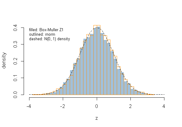
\begin{aligned} Z_1 &= \sqrt{-2\ln U_1}\,\cos(2\pi U_2) \\ Z_2 &= \sqrt{-2\ln U_1}\,\sin(2\pi U_2) \end{aligned}

It is exact but slow, because of the square root, logarithm, sine and cosine. Below, $Z_1$ is drawn against the built-in normal generator and the standard normal density.

Python

U1, U2 = rng.random(5000), rng.random(5000)
Z1 = np.sqrt(-2 * np.log(U1)) * np.cos(2 * np.pi * U2)
Z2 = np.sqrt(-2 * np.log(U1)) * np.sin(2 * np.pi * U2)
print(f"Z1: mean {Z1.mean():.3f}, sd {Z1.std():.3f} | Z2: mean {Z2.mean():.3f}, sd {Z2.std():.3f} | correlation {np.corrcoef(Z1, Z2)[0, 1]:.3f}")
Z3 = rng.standard_normal(5000)
z = np.linspace(-4, 4, 200)
fig, ax = plt.subplots(figsize=(6, 4.2))
ax.hist(Z1, bins=40, density=True, alpha=0.5, label="Box-Muller Z1")
ax.hist(Z3, bins=40, density=True, histtype="step", linewidth=1.5, label="numpy standard_normal")
ax.plot(z, np.exp(-z**2 / 2) / np.sqrt(2 * np.pi), "k--", label="N(0, 1) density")
ax.set(xlabel="z", ylabel="density")
ax.legend(fontsize=8)
plt.show()
print("share within 1.96 of 0:", np.mean(np.abs(Z1) < 1.96).round(3), "(Box-Muller),", np.mean(np.abs(Z3) < 1.96).round(3), "(numpy)")

Z1: mean -0.022, sd 1.002 | Z2: mean -0.011, sd 1.012 | correlation 0.004

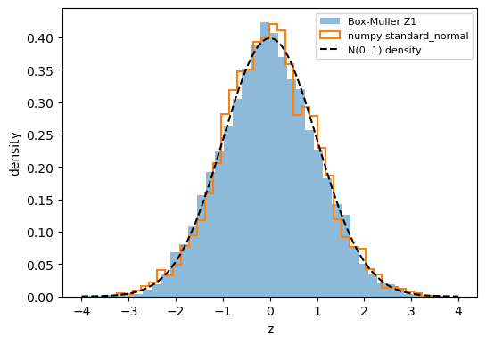
The filled Box-Muller histogram and the outlined numpy histogram both follow the dashed bell curve of the standard normal, peaking near 0.4 at z = 0, and about 95% of each sample lies within 1.96 of zero.

share within 1.96 of 0: 0.949 (Box-Muller), 0.946 (numpy)

U1 <- runif(5000); U2 <- runif(5000)
Z1 <- sqrt(-2 * log(U1)) * cos(2 * pi * U2)
Z2 <- sqrt(-2 * log(U1)) * sin(2 * pi * U2)
cat(sprintf("Z1: mean %.3f, sd %.3f | Z2: mean %.3f, sd %.3f | correlation %.3f\n", mean(Z1), sd(Z1), mean(Z2), sd(Z2), cor(Z1, Z2)))
Z3 <- rnorm(5000)
hist(Z1, breaks = 40, freq = FALSE, col = adjustcolor("steelblue", 0.5), border = "white",
     xlim = c(-4, 4), main = "", xlab = "z", ylab = "density")
hist(Z3, breaks = 40, freq = FALSE, col = NA, border = "darkorange", add = TRUE)
curve(dnorm(x), from = -4, to = 4, lty = 2, lwd = 1.5, add = TRUE)
text(-4, 0.4, "filled: Box-Muller Z1\noutlined: rnorm\ndashed: N(0, 1) density", adj = c(0, 1), cex = 0.8)
cat("share within 1.96 of 0:", round(mean(abs(Z1) < 1.96), 3), "(Box-Muller),", round(mean(abs(Z3) < 1.96), 3), "(rnorm)\n")

Z1: mean -0.033, sd 1.001 | Z2: mean -0.012, sd 0.981 | correlation 0.004
share within 1.96 of 0: 0.951 (Box-Muller), 0.949 (rnorm)

The filled Box-Muller histogram and the outlined rnorm histogram both follow the dashed bell curve of the standard normal, peaking near 0.4 at z = 0, and about 95% of each sample lies within 1.96 of zero.

Counting trials: geometric and negative binomial

Repeat Bernoulli( $p$ ) trials until the first success; $K$ is the number of failures plus the one success. With $p = 0.2$ , the mean is $1/p = 5$ .

numpy's geometric counts trials the same way.

R's rgeom counts only the failures, so add 1 to compare.

Python

p = 0.2
K = []
for rep in range(10_000):
    k = 1
    while rng.random() > p:
        k += 1
    K.append(k)
print(f"built geometric: mean {np.mean(K):.3f} | numpy: {rng.geometric(p, 10_000).mean():.3f} | 1/p = {1 / p}")

built geometric: mean 4.876 | numpy: 5.017 | 1/p = 5.0

p <- 0.2
K <- replicate(10000, {
  k <- 1
  while (runif(1) > p) k <- k + 1
  k
})
cat(sprintf("built geometric: mean %.3f | rgeom + 1: %.3f | 1/p = %.1f\n", mean(K), mean(rgeom(10000, p) + 1), 1 / p))

built geometric: mean 4.982 | rgeom + 1: 4.994 | 1/p = 5.0

Keep going until $r = 2$ successes and count all the trials: negative binomial, mean $r/p = 10$ .

numpy's negative_binomial counts only the failures, so add $r$ to compare.

R's rnbinom counts only the failures, so add $r$ to compare.

Python

r = 2
trials = []
for rep in range(10_000):
    successes, k = 0, 0
    while successes < r:
        k += 1
        if rng.random() <= p:
            successes += 1
    trials.append(k)
print(f"built: mean {np.mean(trials):.3f} | numpy + r: {(rng.negative_binomial(r, p, 10_000) + r).mean():.3f} | r/p = {r / p}")

built: mean 9.985 | numpy + r: 9.905 | r/p = 10.0

r <- 2
trials <- replicate(10000, {
  successes <- 0
  k <- 0
  while (successes < r) {
    k <- k + 1
    if (runif(1) <= p) successes <- successes + 1
  }
  k
})
cat(sprintf("built: mean %.3f | rnbinom + r: %.3f | r/p = %.1f\n", mean(trials), mean(rnbinom(10000, r, p) + r), r / p))

built: mean 10.057 | rnbinom + r: 9.875 | r/p = 10.0

Queueing metrics

The usual measures of a queue, which carry over to most simulations:

$L$ : average number of jobs in the system; $L_q$ : average number waiting in the queue
$W$ : average time a job spends in the system; $W_q$ : average time waiting in the queue
utilisation (share of time the server is busy) and throughput (jobs finished per unit time)
the distributions of waiting time, system size and queue size, not just their averages

For an M/M/1 queue (exponential arrivals at rate $\lambda$ , one exponential server at rate $\mu$ , $\rho = \lambda/\mu < 1$ ) the averages have formulas. A busy period (from an arrival at an empty system until it next empties) also has a mean:

\begin{aligned} L &= \frac{\rho}{1 - \rho} \\ W &= \frac{L}{\lambda} = \frac{1}{\mu - \lambda} \\ \text{mean busy period} &= \frac{1}{\mu - \lambda} \end{aligned}

With $\lambda = 0.3$ and $\mu = 1$ : $\rho = 0.3$ , $L = 0.3/0.7 \approx 0.4286$ , and $W$ and the mean busy period are both $1/0.7 \approx 1.4286$ .

An M/M/1 queue, simulated

Simulate it event by event. With $n$ jobs present, the next event comes after an exponential time at rate $\lambda + \mu$ (or $\lambda$ if the system is empty), and it is an arrival with probability $\lambda/(\lambda + \mu)$ . Between events, add $n \times$ (time elapsed) to a running area; the area divided by the clock is the time-average $L$ . Run to time 500, ten times. Predict: will all ten estimates of $L$ land within 0.1 of 0.4286?

Python

lam, mu = 0.3, 1.0
rho = lam / mu
horizon, reps = 500, 10
L_sim, busy_share, busy_period = [], [], []
for rep in range(reps):
    clock, n_jobs, area, busy, n_busy_periods = 0.0, 0, 0.0, 0.0, 0
    while clock < horizon:
        rate = lam + mu if n_jobs > 0 else lam
        dt = rng.exponential(1 / rate)
        area += n_jobs * dt
        if n_jobs > 0:
            busy += dt
        clock += dt
        if n_jobs == 0:
            n_jobs, n_busy_periods = 1, n_busy_periods + 1    # an arrival starts a busy period
        elif rng.random() < lam / rate:
            n_jobs += 1                                       # an arrival
        else:
            n_jobs -= 1                                       # a departure
    L_sim.append(area / clock)
    busy_share.append(busy / clock)
    busy_period.append(busy / n_busy_periods)
print("L from each run:", np.round(L_sim, 3))

L from each run: [0.259 0.359 0.383 0.523 0.451 0.46  0.496 0.473 0.455 0.391]

lam <- 0.3; mu <- 1
rho <- lam / mu
horizon <- 500; reps <- 10
L_sim <- busy_share <- busy_period <- numeric(reps)
for (rep in 1:reps) {
  clock <- 0; n_jobs <- 0; area <- 0; busy <- 0; n_busy_periods <- 0
  while (clock < horizon) {
    rate <- if (n_jobs > 0) lam + mu else lam
    dt <- rexp(1, rate)
    area <- area + n_jobs * dt
    if (n_jobs > 0) busy <- busy + dt
    clock <- clock + dt
    if (n_jobs == 0) {
      n_jobs <- 1; n_busy_periods <- n_busy_periods + 1    # an arrival starts a busy period
    } else if (runif(1) < lam / rate) {
      n_jobs <- n_jobs + 1                                 # an arrival
    } else {
      n_jobs <- n_jobs - 1                                 # a departure
    }
  }
  L_sim[rep] <- area / clock
  busy_share[rep] <- busy / clock
  busy_period[rep] <- busy / n_busy_periods
}
cat("L from each run:", round(L_sim, 3), "\n")

L from each run: 0.358 0.478 0.416 0.509 0.263 0.269 0.539 0.383 0.299 0.512

Now the averages over the ten runs beside the formulas. $W$ comes from Little's law, $W = L/\lambda$ , applied to each run.

Python

pd.DataFrame({
    "formula": [rho / (1 - rho), 1 / (mu - lam), rho, 1 / (mu - lam)],
    "simulated (mean of 10)": [np.mean(L_sim), np.mean(L_sim) / lam, np.mean(busy_share), np.mean(busy_period)],
    "sd across runs": [np.std(L_sim, ddof=1), np.std(L_sim, ddof=1) / lam, np.std(busy_share, ddof=1), np.std(busy_period, ddof=1)],
}, index=["L", "W", "utilisation", "mean busy period"]).round(4)

	formula	simulated (mean of 10)	sd across runs
L	0.4286	0.4249	0.0778
W	1.4286	1.4164	0.2592
utilisation	0.3000	0.3015	0.0444
mean busy period	1.4286	1.4268	0.1933

round(data.frame(
  "formula" = c(rho / (1 - rho), 1 / (mu - lam), rho, 1 / (mu - lam)),
  "simulated (mean of 10)" = c(mean(L_sim), mean(L_sim) / lam, mean(busy_share), mean(busy_period)),
  "sd across runs" = c(sd(L_sim), sd(L_sim) / lam, sd(busy_share), sd(busy_period)),
  row.names = c("L", "W", "utilisation", "mean busy period"), check.names = FALSE
), 4)

                 formula simulated (mean of 10) sd across runs
L                0.4286  0.4028                 0.1043        
W                1.4286  1.3426                 0.3478        
utilisation      0.3000  0.2846                 0.0563        
mean busy period 1.4286  1.3395                 0.2372

Monte Carlo integration

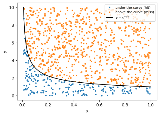
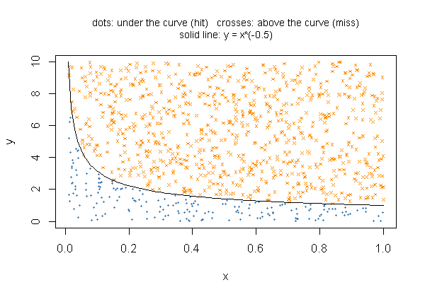
Estimate $\int_{0.01}^{1} x^{-0.5}\,dx$ (exactly $2(1 - 0.1) = 1.8$ ) by throwing points into a box and counting the share that land under the curve. The box spans $x$ from 0.01 to 1 and $y$ from 0 to the function's largest value on that range, found on a grid as before. Predict: with 1,000 points, how far from 1.8 will the estimate be?

Python

a, b = 0.01, 1.0
height = (np.linspace(a, b, 10_001) ** -0.5).max()
x = rng.uniform(a, b, 1000)
y = rng.uniform(0, height, 1000)
hit = y < x ** -0.5
print(f"box height {height:.2f} | hits {hit.sum()} of 1000 | estimate {(b - a) * height * hit.mean():.4f} | exact 1.8")
fig, ax = plt.subplots(figsize=(6, 4.2))
ax.scatter(x[hit], y[hit], s=6, marker="o", label="under the curve (hit)")
ax.scatter(x[~hit], y[~hit], s=8, marker="x", label="above the curve (miss)")
xs = np.linspace(a, b, 300)
ax.plot(xs, xs ** -0.5, "k-", label=r"$y = x^{-0.5}$")
ax.set(xlabel="x", ylabel="y")
ax.legend(fontsize=8)
plt.show()

box height 10.00 | hits 195 of 1000 | estimate 1.9305 | exact 1.8

Of 1,000 random points in the box from x = 0.01 to 1 and y = 0 to 10, the 195 dots under the steep curve y = x^-0.5 sit in a thin band along the bottom and a spike at the far left, while the crosses above the curve fill the rest of the box.

a <- 0.01; b <- 1
height <- max(seq(a, b, length.out = 10001)^-0.5)
x <- runif(1000, a, b)
y <- runif(1000, 0, height)
hit <- y < x^-0.5
cat(sprintf("box height %.2f | hits %d of 1000 | estimate %.4f | exact 1.8\n", height, sum(hit), (b - a) * height * mean(hit)))
plot(x[hit], y[hit], pch = 16, cex = 0.4, col = "steelblue", xlim = c(a, b), ylim = c(0, height), xlab = "x", ylab = "y")
points(x[!hit], y[!hit], pch = 4, cex = 0.5, col = "darkorange")
curve(x^-0.5, from = a, to = b, add = TRUE)
title(main = "dots: under the curve (hit)   crosses: above the curve (miss)\nsolid line: y = x^(-0.5)", cex.main = 0.85, font.main = 1)

box height 10.00 | hits 189 of 1000 | estimate 1.8711 | exact 1.8

Of 1,000 random points in the box from x = 0.01 to 1 and y = 0 to 10, the 189 dots under the steep curve y = x^-0.5 sit in a thin band along the bottom and a spike at the far left, while the crosses above the curve fill the rest of the box.

The same idea for a semicircle: $\int_{-1}^{1}\sqrt{1 - x^2}\,dx$ is half the area of the unit circle, $\pi/2$ . The box height is the function's largest value on the range, rounded up. Use a million points this time.

Python

a, b = -1.0, 1.0
height = np.ceil(np.sqrt(1 - np.linspace(a, b, 2001) ** 2).max())
x = rng.uniform(a, b, 1_000_000)
y = rng.uniform(0, height, 1_000_000)
estimate = (b - a) * height * np.mean(y < np.sqrt(1 - x ** 2))
print(f"box height {height:g} | estimate {estimate:.5f} | pi/2 = {np.pi / 2:.5f}")

box height 1 | estimate 1.57148 | pi/2 = 1.57080

a <- -1; b <- 1
height <- ceiling(max(sqrt(1 - seq(a, b, length.out = 2001)^2)))
x <- runif(1e6, a, b)
y <- runif(1e6, 0, height)
estimate <- (b - a) * height * mean(y < sqrt(1 - x^2))
cat(sprintf("box height %g | estimate %.5f | pi/2 = %.5f\n", height, estimate, pi / 2))

box height 1 | estimate 1.57155 | pi/2 = 1.57080

Questions

The ten simulated values of $L$ are spread out even though the model never changes. Would running one simulation to time 5,000 or ten to time 500 give you a better estimate, and why?
Raise $\lambda$ to 0.9 in the queue and rerun. What happens to $L$ and to the spread across runs?
Acceptance-rejection threw away about half its candidates. What would happen to that share if $c$ were set larger than the true maximum, and would the kept values still be Beta(2, 4)?

Going further: the Monte Carlo and simulation notebook in the lab's teaching library.